Table of Contents

LIST OF Tables

LIST OF Figures

List of Abbreviations and Symbols

Acknowledgements

Abstract

(click on the '*' to jump to a section)

1. Introduction *

1.1. Objectives *

1.2. Scope *

1.3. Location *

1.4. History *

1.5. Regional Geology *

1.6. Poura Mine Geology *

1.7. Literature Review *

2. Geostatistical Theory *

2.1. Regionalised Variables and Random Functions *

2.2. Stationarity *

2.3. The Covariance Function or Variogram *

2.4. Nugget Effect *

2.5. Linear Estimators *

2.6. Regularization *

2.6.1. Regularizing Over a Constant Thickness *

2.7. Calculating Semi-Variograms *

2.8. Grade Estimation *

2.9. Change in Support (Block Kriging) *

2.10. Optimising Sample Spacing *

2.11. Drift *

3. Analysis of Provided Data *

3.1. Supplied Data *

3.2. Statistical Analysis *

3.3. Data Preparation *

3.4. Changes *

3.5. Regularization *

3.6. Grade and Vein Thickness Semi-variogram Modeling *

4. Development of Kriging Methodology *

4.1. Justification of Approach *

4.2. Krige2D *

4.3. Verifying Krige2D *

4.4. Krige2D Input *

4.5. Observations *

4.5.1. Point Spacing *

4.5.2. Block Areas *

5. Resource Estimation Results and Discussion *

5.1. Using Confidence Limits in Risk Analysis *

5.2. Kriging Resources (no Cut-off Grade Considered) *

5.3. Comparison Between Kriging Resources and ACA Howe’s Resources *

5.4. Cut-off Grades *

5.5. Comparing Geostatistical and Non-geostatistical Methods *

5.6. Exploration Potential *

6. Conclusions and Recommendations *

6.1. Conclusions *

6.2. Recommendations for Future Work *

6.2.1. Using Confidence Limits in Making a Production Decision *

6.2.2. Expected Profit *

References
 
 
 
 

List of Tables

Table 3-1: Sample statistics. *

Table 3-2: Samples for which coordinates could not be assigned. *

Table 3-3: Diamond drill holes that previously had not been considered and were not part of the supplied data set. *

Table 3-4: Number of sample pairs for each lag interval for the four principal directions. *

Table 5-1: Summary statistics of kriging results. *

Table 5-2: Overall kriging resources (variances not considered). *

Table 5-3: Comparison between kriging resources and those that were estimated by ACA Howe. *

Table 5-4: Resources considering cut-off grades and confidence in grade and vein thickness using a 50 % lower limit of confidence. *

Table 6-1: Fictional example of the results of a profitability analysis using confidence limits. *
 
 
 
 

List of Figures

Figure 1-1: Location map (CIA, 1987). *

Figure 1-2: Longitudinal section of the Poura Mine. *

Figure 2-1: Relationship between the covariance function and semi-variogram. *

Figure 2-2: Effect of sample configuration on estimation variance.. *

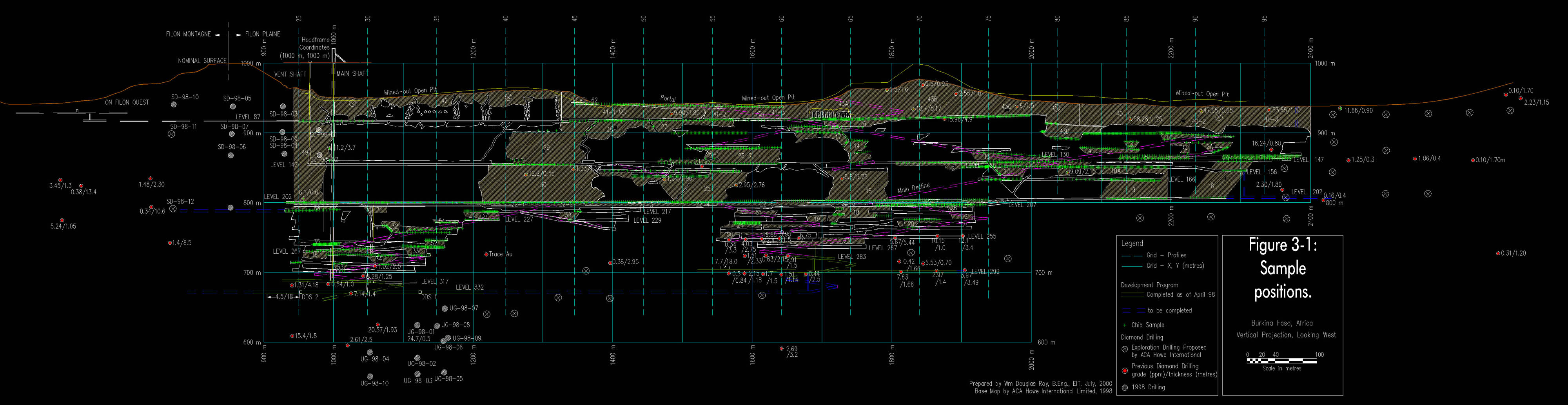
Figure 3-1: Sample positions. *

Figure 3-2: Grade histogram and cumulative distribution. *

Figure 3-3: Grade histogram with cumulative distribution, plotted with a logarithmic x-axis. *

Figure 3-4: Vein thickness histogram and cumulative distribution *

Figure 3-5: Vein thickness semi-variogram experimental data and fitted spherical model for search azimuth 90° +/-22.5° (along strike). *

Figure 3-6: Grade semi-variogram data and fitted models for search azimuth 90° +/- 22.5° (along strike). *

Figure 3-7: Vein thickness semi-variogram data for search azimuth 0° +/- 22.5° (along dip). *

Figure 3-8: Vein thickness semi-variogram data for search azimuth 45° +/- 22.5° (south plunging). *

Figure 3-9: Vein thickness semi-variogram data for search azimuth 135° +/- 22.5° (north plunging). *

Figure 3-10: Grade semi-variogram data for search azimuth 0° +/- 22.5° (along dip). *

Figure 3-11: Grade semi-variogram data for search azimuth 45° +/- 22.5° (south plunging).. *

Figure 3-12: Grade semi-variogram data for search azimuth 135° +/- 22.5° (north plunging). *

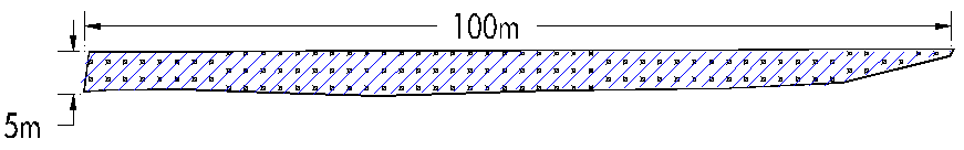
Figure 4-1: Test stopes for confirming Krige2D's results. *

Figure 4-2: A portion of Block 22 showing the block kriging internal grid points *

Figure 4-3: Block 7 showing internal points at a two metre spacing. *

Figure 5-1: Estimated grade accumulation (grade x thickness). *

Figure 5-2: Probability plot for a mean grade of 20 g/tonne and a standard deviation of 5 g/tonne. *

Figure 5-3: Probability plot for a mean grade of 20 g/tonne and a standard deviation of 5 g/tonne. *

Figure 5-4: Grade-tonnage curve showing resource quantity and average grade using a 50 % lower limit of confidence. *

Figure 5-5: Grade-tonnage curve showing resource quantity and average grade using several lower limits of confidence. *

Figure 5-6: Grade-tonnage curve showing resource quantity and average grade using a lower limit of confidence equal to 84 %. *
 
 
 
 

List of Abbreviations and Symbols

Symbol Explanation

$CA  Canadian Dollars

$US  United States Dollars

° degrees (angle)

+/- plus or minus

two-dimensional matrix K

one dimensional matrix b

S summation

b sample weight

g (h) variance at a lag h

s standard deviation

s ² variance

m Lagrange parameter

a range (metres)

A area

Au gold

° C degrees in Celsius

C covariance

C_o maximum covariance

Eq. Equation

E{Z} expected value of Z

g/tonne grams of gold per tonne of rock

h lag (metres)

kg kilogram

km kilometre

m metre

NPV Net Present Value

ppm parts of gold per million parts of rock

tonne one thousand kilograms

toz troy ounce (1/12^th of a pound)

V volume

Z* estimator of Z
 
 

Acknowledgements

This investigation was made possible with the aid of Dr. Stephen Butt, Assistant Professor with the Mining and Metallurgical Engineering Department at DalTech, Dalhousie University. Dr. Butt acted as Thesis Supervisor and, in that role, provided general direction. More specifically, he was an excellent source of computer programming knowledge during the writing of Krige2D. Dr. D. H. Steve Zou, Professor and Mining Graduate Coordinator with the Mining and Metallurgical Department at DalTech, provided technical advice and general guidance. Dr. Gordon Fenton, Professor in the Engineering Mathematics Department at Dalhousie University, assisted with kriging theory and also provided direction during the writing of Krige2D. Two of his subroutines for solving matrices, Dgselu and Dnsolv, were used in Krige2D with his permission. Mr. Patrick Hannon, President of MineTech International Limited, provided invaluable site information. Sahelian International Goldfields, the Poura Mine’s current owner, graciously allowed the use of sampling data and their 1998 feasibility report. The Faculty of Graduate Studies partially funded this investigation through a Graduate Student Award for the 1999/2000 year of studies. The author thanks everyone involved for making this investigation possible.
 
 

Abstract

Because of its dependence on computers, geostatistics has been criticised as being a black-box approach to grade estimation. Though geostatistical resource estimations are becoming more common, there is a widespread lack of understanding of the method’s mechanics. The objectives of this investigation were to carry out a geostatistical resource estimate for the Poura deposit and to increase the industry’s awareness and understanding of geostatistical methods.

The Poura Mine in Burkina Faso, West Africa consists of steeply-dipping, gold-silver mineralized quartz veins. The structure has a strike length of two kilometres and an average vein thickness of about two metres. This resource estimate concentrated on the remnant ore blocks and pillars in the underground workings.

Using the supplied information, coordinates were assigned to 3,232 samples. Semi-variograms were calculated for grade and vein thickness. The raw data followed clear trends to which models could readily be fit. Ordinary block kriging was chosen as the appropriate kriging method. The author wrote a block kriging computer program called Krige2D to carry out the kriging calculations. For each block, the estimated grade and variance, as well the estimated vein thickness and variance, were calculated using Krige2D.

The undiluted, mean block grade ranged between 4.7 g/tonne and 36.3 g/tonne with variance ranging between 9.4 (g/tonne)² and 143 (g/tonne)². Estimated thickness ranged from 0.77 metres to 3.81 metres. Thickness variance ranged between 0.0014 m² and 0.37 m². The mean grade was used to calculate the remnant block resources. When no cut-off grade is considered, undiluted resources consist of 468,000 tonnes with an average grade of 14.8 g/tonne. The resource contains a total of 6.95 tonnes (220,000 troy ounces) of gold and has an average vein thickness of 1.86 metres. Using a cut-off grade of 5.0 g/tonne, the resource consists of 464,000 tonnes with an average grade of 14.9 g/tonne.

A previous resource estimate had been carried out using arithmetic methods. Block kriging estimated the average grade to by 2.5 g/tonne higher and the total amount of gold to be 1.2 tonnes higher. When confidence in the estimate and a 5.0 g/tonne cut-off grade were considered, the undiluted resource drops from 464,000 tonnes to 367,000 tonnes (a 21 % decrease) when the confidence in the estimate is increased from 50 % (mean value) to 70 %. The average grade decreases from 14.9 g/tonne to 13.5 g/tonne (a 9 % decrease).

Additional work is warranted. An economic analysis should be carried out. Block kriging should be used with that economic analysis to optimise the sample spacing of future exploration programs. Further exploration is recommended along strike and down dip the current workings.
 
 

1. Introduction

The Poura Mine in Burkina Faso, West Africa has mined a narrow vein gold deposit using modern open pit and underground mining methods since the early 1980’s. Previous resource estimating practices did not make use of geostatistics. In 1998, a feasibility study was carried out for the remnant ore blocks that consist of pillars and ‘lower grade’ ore blocks that remain in the underground mine. That study made use of an arithmetic resource estimation method. This thesis extends that initial work by using geostatistics to further define Poura’s resources.
 
 

1.1 Objectives

The objectives of this thesis were to:

• use geostatistics to estimate the Poura deposit’s resources; and,
• increase the mineral industry’s awareness and acceptance of geostatistical methods.

1.2 Scope

The scope of this investigation included:

• calculating sample coordinates;
• analysing the sample statistics;
• writing a block kriging computer program and confirming its accuracy;
• carrying out structural analyses for grade and thickness;
• calculating each block’s estimated mean grade and thickness;
• computing the deposit’s ‘overall’ resources;
• exploring how cut-off grade and confidence affect those resources; and,
• discussing how the previous item could be used in an economic analysis to determine the project’s profitability.

1.3 Location
The Poura mine is located in the Mouhoun Province of southwestern Burkina Faso (Figure 1-1). It has an area of 500 km² and is centered over 11° 35’ North Latitude and 2° 45’ West Longitude. Poura is about 180 kilometres southwest of the capital Ouagadougou.

The site is accessed from the capital via paved highway to within 20 kilometres of the site. The final segment is lateritic road. Site topography is uneven with relief of up to tens of metres (Titaro and Hannon, 1998). The area drains into the Mouhoun River (Black Volta). The average rainfall is 900 millimetres, with about 250 millimetres falling in August – the rainy season. The temperature varies between 15 ° C and 45 ° C.
 
 

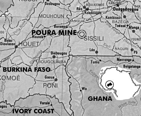
Figure 1-1: Location map (CIA, 1987).
 

1.4 History
Gold mining has a long history in West Africa that predates Western influence (Titaro and Hannon, 1998). Artisanal miners (orpailleurs) exploited Poura’s mineral resources long before a modern mine was established in 1939. They exploited auriferous quartz veins, paleo placers, and lenses of disseminated mineralisation. Between 1939 and 1944, a French company used a small mill for reprocessing the orpailleur tailings. Another company continued that work in 1949. Both companies extracted about 250 kg of gold.

From 1949 to 1961, a French syndicate explored the deposit using 80 holes, totaling 4,400 metres, along a 750 metre strike length. They tested the vein to 160 metres depth and sank exploration pits. In 1961, underground mining began using shrinkage stoping. Operations ceased in 1966 for economic reasons. In total, 5,600 kg of gold was produced from 420,000 tonnes of treated ore.

Reconnaissance work in 1974 revealed 1.6 million tonnes of ore with an average grade of 13.5 g/tonne. In 1977, a feasibility study was completed that recommended re-opening the mine with the objective of exploiting those underground reserves. After another round of intensive exploration, consisting of 8,795 metres of drilling to the 327 metre level, open pit mining started in 1981. Concurrently, two parallel declines were started that ran to the 147 metre level. They were later extended to the 207 metre level. The mill was commissioned in October 1984.

The open pits were exhausted by 1988. Through poor planning, the open pit broke through one of the declines, causing its collapse. Between 1988 and 1994, the average grade declined from 13.6 g/tonne to 6.4 g/tonne. Deep exploration resumed in 1992. Thirty-nine holes were drilled with an aggregate length of 6,056 metres. In 1995, International Gold Resources (IGR) carried out an extensive exploration program with the aid of the European Union. Ashanti Goldfields took IGR over in 1996 and optioned the mine to Sahelian International Goldfields (Sahelian), the project’s current owner, in 1997. Sahelian continued underground exploration and rehabilitated the surface facilities. In 1998, Sahelian retained ACA Howe International to carry out a feasibility study regarding mining the remnant blocks and pillars in the underground workings (shown in Figure 1-2).
 
 

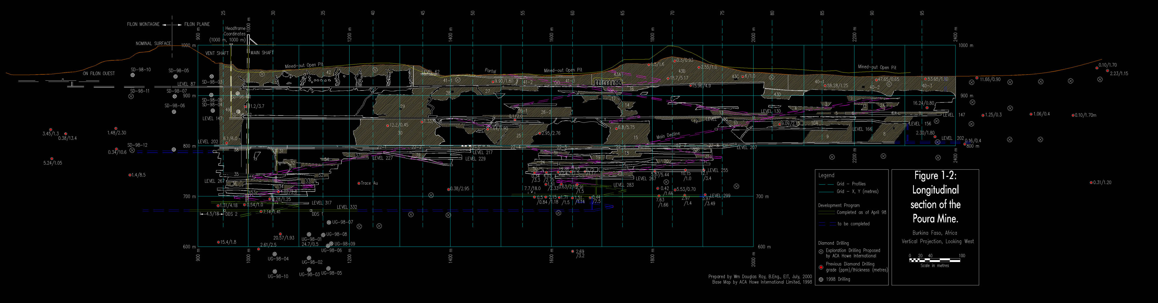
Figure 1-2: Longitudinal section of the Poura Mine.
 
 

1.5 Regional Geology
The Archean Mossi Gneissic-Migmatitic Shield underlies much of Burkina Faso. The Shield includes the gold bearing, Birimian-age (Proterozoic) greenstone belts. The Poura mine is in the center of the Boromo-Goren greenstone belt that strikes in a northerly to northeasterly direction. It consists of andisitic/dacitic volcanics, volcano-sedimentaries such as tuff and agglomerate, and detrital sedimentary formations consisting of pelitic to conglomeratic rocks. A regional northerly foliation is present in the sedimentary rocks. Felsic to mafic intrusions, granitic to gabbroic in texture, are metamorphosed to greenschist facies.

Several phases of deformation have taken place:

1. Regional and localised folding of the greenstone belt along a northerly trending axis;
2. Easterly folding and shearing that created localized bands of mylonitised rocks; and,
3. Later sinistral faulting, oriented about 155 ° , and intrusion of spatially-related syntectonic rocks.

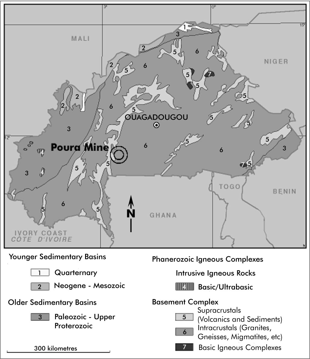
Figure 1-3: Regional geology (European Union, 1998).
 

1.6 Poura Mine Geology
Laterite covers the bedrock with a thickness that ranges from 0.5 metres to about twenty metres. Numerous mining excavations and drill holes provide a view of the bedrock geology that will be described in order from oldest to youngest. The footwall consists of dark green volcaniclastic rocks that are greater than two hundred metres thick. They consist of welded tuffs, lapillis, pyroclastic breccias, and doleritic basalts with veinlets of quartz and rose carbonate.

Younger detrital sedimentary formations, 20-200 metres thick, form the hanging wall. The ore is often fully surrounded by them. They consist of conglomerates, greywackes, sandstones, chert, and pelites. The base consists of conglomerates, sandstones, and greywackes with periodic intercalations of chert. The top consists of banded siltstone-mudstone with typical turbiditic structures.

Volcanic formations, greater than two hundred metres thick, overlie the detrital formations. They consist of massive andesite flows, ash tuffs, lapilli tuffs, pyroclastic breccias, agglomerates, and volcanic dikes that cut the agglomerates.

The ore consists of three principal steeply-dipping quartz veins. These are the Filon Plaine, Filon Montagne, and Filon Ouest. There are also several minor related veins. Filon Plaine is the most economically important and is the focus of current production.

Filon Plaine has a strike length of about two thousand metres. It is oriented southeast 150 ° with an average dip of 70 ° southwest. Its thickness ranges from several centimetres to eight metres with an average thickness of two metres. The vein continues to a depth of at least 400 metres with a thickness ranging from several centimetres to 3.5 metres. The wall rock is altered where it contacts the vein. Regional, sinistral faults frequently displace the vein and change its direction. The fault set is oriented 100-120 ° .

The ore is vein quartz with silver-bearing (11 % average silver content) native gold and a minor percentage (about 2 %) of polymetallic sulphides. The deposit is oxidised (weathered) down to one hundred metres depth by supergene alteration that also produced locally high gold grades.

The ore is made up of several different types. There is low-grade milky, massive white quartz. There is also grey vein quartz within the massive white quartz vein that is rich in pyrite-associated gold. A third type is heterogeneous milky white quartz that is present in the sinistral fractures. That type is barren of gold. The final type is boxwork quartz in the upper one hundred metres of the deposit where the gold was leached and concentrated. The boxwork quartz has the highest grades of all the ore types.

Most of the gold is free-milling, but minor a small percentage is locked in the sulphides (refractory). Gold mineralisation occurs in ore shoots that plunge 50-70 ° towards the south. Below 100 metres depth (supergene enrichment zone), the shoots laterally extend 150-250 metres and have a height of 200-250 metres.
 

1.7 Literature Review
The use of geostatistics essentially began in the early to mid-1970’s when computers were starting to become available. In the 1980’s and 1990’s when computers became common, much work was carried out in the field of geostatistics. However, geostatistics is most often applied to relatively larger and more uniform deposits (Sinclair and Deraisme, 1974). The often erratic mineralisation of vein deposits often disqualifies the use of geostatistics for reasons that will be described in later paragraphs. The vast majority of resource estimates concerning vein deposits that are reported in the literature did not make use of geostatistics.

Many more papers have been reviewed than are reported in this section; however, they will not be mentioned because either they did not pertain to vein deposits or an estimating method other than geostatistics was used. One reason why geostatistics is often not used is because vein deposits, especially precious metals vein deposits, are often characterised by a skewed grade distribution. Extreme values or ‘outliers’ can cause the grade of a point or block to be overestimated (Kim et al, 1987; Dominy et al, 1997). They can also cause distortions, such as pure nugget effect, in variograms that render them useless (Kim et al, 1987).

Another reason for not choosing geostatistics for estimating the resources of a vein deposit has to do with the relative importance of choosing the most correct type of estimating method. Correctly estimating the grade of a resource is crucial. However, when the subject of the estimate is a vein deposit, the errors that make the most impact on a resource estimate are generally made in defining the geometry of the orebody (Deutsh, 1989; Dominy et al, 1997). By that it is not implied that the choice and accuracy of the grade estimating method is unimportant; rather, correctly defining a vein deposit’s geometry is paramount for estimating resources. Because of that, evaluators are more likely to choose less complicated methods such as inverse distance weighting or graphical methods.

With non-geostatistical methods, the extreme values are most often dealt with by ‘cutting’ them to a certain value (Deutsh, 1989; Dominy et al, 1997, Fytas et al, 1990). In operating mines, the cut value is generally arrived at through experience (Dominy et al, 1997; Fytas et al, 1990). In the absence of such information as is generally the case prior to production, there are several commonly used cut values. One method used in gold deposits consists of limiting the sample values to a grade of one troy ounce per ton (Dominy et al, 1997). Another method consists of limiting the grade to a value equal to the sample average plus one or two standard deviations. Yet another method consists of limiting samples to the value where the ragged tail begins on a sample histogram. The objective of cutting the high-grade samples is to change the sample distribution so that the average grade will not be overestimated. However, such manipulations can lead to errors in estimation, usually by underestimating the grade and over-estimating the quantity of material (Fytas et al, 1990).

As previously mentioned, skewed grade distributions, such as those that are often found in precious metals vein deposits, can hinder the use of geostatistics. The erratic mineralisation can cause the variogram to be ‘pure nugget’ – essentially useless from a geostatistical standpoint (Dominy et al, 1997). Also, like non-geostatistical methods (though not as severely), ordinary kriging sometimes overestimates the grade in skewed distributions. Several kriging methods were developed to resolve that problem, including lognormal kriging (Armstrong and Boufassa, 1988), outlier restricted kriging (Arik, 1992), indicator kriging (Fytas et al, 1990; Journel, 1983; Journel, 1984; Kwa and Mousset-Jones, 1986), probability kriging (closely related to indicator kriging) (Journel, 1985; Verly and Sullivan, 1985), multigaussian kriging (Verly, 1983), and disjunctive kriging (Kim et al, 1977; Jackson and Marechal, 1979). As one would expect, those methods are much more complicated, more time-consuming, and therefore more expensive, than ordinary kriging.

Several authors (Dominy et al, 1997; Fytas et al, 1990) have stated that for grade distributions with a coefficient of variation (standard deviation divided by the average) of less than about 1.5, meaningful variograms can be produced. Fytas et al (1990) also stated that parametric geostatistics (ordinary kriging) performs well in deposits with a coefficient of variation close to (or less than) one.

Sinclair and Deraisme (1974) used ordinary block kriging to estimate the resources of the Eagle Copper Vein in British Columbia. The sulphide-mineralised quartz vein averages about 1.2 metres thick. The sulphide mineralisation consists of chalcopyrite (80-95 %), pyrite, and a small amount of covellite. Two parameters were estimated: vein thickness and accumulation (thickness x grade). Both parameters appeared to be lognormally distributed, indicating skewed distributions. All of the samples were taken along three parallel, horizontal drifts. Therefore, variograms could only be prepared for the horizontal direction. It was therefore assumed that the variogram was isotropic. The kriging problem was simplified to two dimensions. To accomplish that, the vein was ‘unfolded’ or ‘flattened’ by defining horizontal and vertical positions as the distance along the vein from a certain origin.

Tulcanaza (1972) presented a case where ordinary block kriging was used to estimate the resources of the Uchucchacua argentiferous vein. The mineralisation consisted of argentiferous pyrite with a minor amount of galena. The steeply dipping vein was displaced by faulting along the vertical direction. Chip samples were taken at one metre intervals along drifts and raises. The variogram structure was determined to be anisotropic. The variogram range in the vertical direction was 20 metres, while the range in the horizontal direction was 70 metres. For kriging, sets of samples were regularized into mean grades for segments of drifts and raises. A correction term was added to the kriging variance to account for the change in support.

Kim et al (1987) compared the results of ordinary kriging and indicator kriging against production results from a large, low grade, Carlin type, open pit, gold-silver orebody in Nevada. The grade distribution was highly skewed and no useable variograms could be obtained from the raw grade data. However, grade variograms were obtained from the logarithms of the samples. The authors concluded that the results of indicator kriging were similar to actual production results. However, ordinary kriging overestimated the gold quantity by about twenty-five percent.

Even though the variance allows the evaluator to explore the confidence of the estimate, reports of those activities in the literature are rare. Most of the numerous published papers that were reviewed during this investigation failed to go beyond the end stage of kriging. In other words, resources were estimated, but the estimation variance was not used to investigate the confidence in those resources. A thorough description of how such a risk analysis could be carried out could not be found either. This investigation will strive to resolve those two deficiencies.
 
 
 

2. Geostatistical Theory

During kriging, each sample is assigned a sample weight. The weighted samples are then linearly combined to give the best estimate. It is the ‘best’ estimate because the procedure minimises the expected error between the estimated grade and the true grade. Sample weights are calculated such that the variance of the estimate is a minimum. That variance can be calculated using the sample positions and the variogram function. Having the estimation variance is extremely useful because it allows the user to explore the risk of the estimate.
 

2.1 Regionalised Variables and Random Functions
Regionalised variables are variables that are distributed throughout a space (Journel and Huijbregts, 1978). Many variables in the earth sciences, such as those from forestry, agriculture, and geology, are regionalised. For mining application, there are two characteristics that are evident in a regionalised variable. The first characteristic is a local randomness that gives the impression of a random variable. The second is a general, structural pattern that can be represented by a function. The two can be interpreted probabilistically using random functions.

A sample’s grade can be considered a particular realisation of a random variable. A random function is all possible realisations of that random variable. At a point, a grade is considered a random variable. However, a pair of points that are separated by a distance are independent, but also correlated through a certain spatial structure known as the variogram. Because many grade realisations would be necessary to define the random function at a certain point, certain assumptions must be made. One such assumption concerns deposit homogeneity.
 

2.2 Stationarity
Under strict stationarity, the spatial structure alluded to in Section 2.1 must be invariant under translation (Journel and Huijbregts, 1978). That means the expected mean of the random variable must be constant in any location. In practice, quasi-stationarity is assumed to exist. Under that hypothesis, the spatial structure is assumed invariant for a limited distance known as the range b. The range can be rationalised as the limits of a homogeneous zone in a deposit. Variables separated beyond the range are considered uncorrelated.
 

2.3 The Covariance Function or Variogram
The covariance function is one that describes covariance as a function of variable separation. At zero separation distance, two variables have the maximum covariance C_o. As their separation increases to the range, covariance decreases from C_o following a certain function (Figure 2-1). At a certain distance, the covariance will approximately equal zero. One type of covariance function, common in geostatistics, is known as a transition structure. From zero separation distance to the range, covariance decreases from C_o to zero. Beyond the range, covariance equals zero.

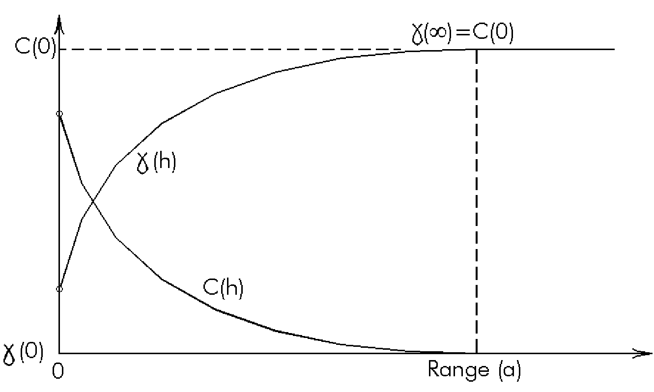
Figure 2-1: Relationship between the covariance function and semi-variogram.
 
 

The variogram function is another way of expressing the degree of covariance between two variables separated by a distance. It is closely related to the covariance function through the following relationship:
 

g (h) = sill + nugget – C(h)         (Eq. 2-1)

where:

g (h) = variance of two variables separated by h distance

sill = the ceiling value for g (h) – nugget value

nugget = value of g (h) very close to h=0 (described later)

C(h) = covariance of two variables separated by h distance

That relationship is shown graphically in Figure 2-1. The covariance structure can be anisotropic, meaning that there can be many different covariance functions that describe the covariance structure along different orientations. For example, variables spaced in the horizontal direction might follow a certain covariance function, while those spaced in the vertical direction might follow another.
 

2.4 Nugget Effect
At a separation distance of zero, two variables have the maximum covariance C_o. The corresponding variogram value g (0)=0, meaning that the variance of two variables located at the same point is equal to zero. The variogram function is discontinuous in that at a very small separation distance, the variogram function equals a certain value known as the nugget value. The nugget value is caused by measurement errors and microvariability in mineralisation (Journel and Huijbregts, 1978). It is a local randomness that is similar to the ‘white noise’ of other phenomena.
 

2.5 Linear Estimators
Generally, when estimating the unknown mean grade Z_v(x) of a block with size V centered over point x from a set of n data values Z(x_i), the grade estimator Z* must be:

• non-biased (E{Z_v-Z*}=0), meaning that the estimated mean must be equal to the true mean;
• simple, to allow calculation of the estimation variance:
s ²_E = E{[Z_v-Z*]²} = E{Z²_V} + E{Z*²} - 2E{Z_VZ*}         (Eq. 2-2)

Suppose that K points x_K are located within a volume V centered on point x and the n points x_i are within another volume v centered on point x’. As K and n tend toward infinity, the arithmetic means of z_K and z_K* tend toward the mean values in V and v of the point variable z(y). The estimation variance s²_E can be written in terms of semi-variograms as:
 

s ²_E = 2(V,v) – (V,V) – (v,v)            (Eq. 2-3)
where:

(V,v) is the mean value of g (h) when one extremity of the vector h describes the domain V(x) and the other extremity describes the domain v(x’).

The preceding equation suggests that as the distance between V and v increases, so does the value of (V,v) and the value of the estimation variance s²_E. Sample configuration is also important. In Figure 2-2, the estimation variance provided by the closely spaced samples in (i) would be greater than that provided by the well-spaced samples in (ii) (formalised by the term [g (v,v)]). That illustrates an important advantage of geostatistics over other estimation methods, such as inverse distance weighting, that would treat both configurations in the same manner.

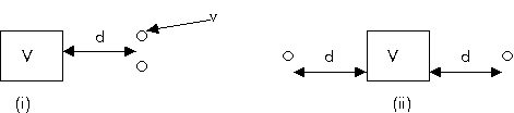
Figure 2-2: Effect of sample configuration on estimation variance. The estimation variance of (i) is greater than that of (ii).
 
 

2.6 Regularization
Samples have a certain volume or support. Statistically, they are considered point grades (a point has no volume) that have been integrated or regularized over the sample volume. It can be shown that the regularized random function Z_v(x) of a second-order stationary point random function is also second-order stationary (Journel and Huijbregts, 1978). Because of stationarity, the expected value of the volume Z_v(x) is identical to the point’s expected value.
 

2.6.1 Regularizing Over a Constant Thickness
When a drill hole or channel sample is taken orthogonally to a horizontal bench or vein, the graded sample grade Z_G is found by integrating the grade over the intersection length and dividing by the length (Journel and Huijbregts, 1978). In the discrete case, that amounts to calculating the weighted average grade (with respect to length) over the vein thickness.

Practically, the regularized semi-variogram is calculated using:

g _l(h) @g (h) - (l,l)                 (Eq. 2-4)

where:
g_l(h) = semi-variogram regularized across thickness l
g (h) = point semi-variogram
(l,l) = constant support term of the thickness l

For a transition model, the above formula is approximate and should be used when the range is greater than three times the vein thickness. To satisfy the positive definite condition that states variance can only be positive or zero, care must be taken when using the formula. If the point semi-variogram g (h) is a spherical model with range a and sill C, the regularized semi-variogram can be built, for distances h less than the thickness l, as a spherical model with:

• Regularized sill C_l = C - (l,l);
• Regularized range:
• a_l = (a + l), if regularization is done using samples of length l; and,
• a_l = a, if regularization is done by grading over a constant thickness l.

2.7 Calculating Semi-Variograms
The variability between two values z(x) and z(x+h) at two points separated by the vector h at x and x+h is described by the variogram function 2g (x,h) that is equal to the expectation:
 

2g (x,h) = E{[Z(x) – Z(x+h)]²}                 (Eq. 2-5)

where: [Z(x) – Z(x+h)] is a random variable

(Journel and Huijbregts, 1978)

To calculate 2g (x,h) properly for a particular separation distance h, we would need several realizations [z(x) – z(x+h)]. In mining applications, only one sample can be taken at a particular position. To bridge that requirement, the intrinsic hypothesis states that the function 2g (x,h) depends only on the separation vector h and not on the position x. Practically, the function 2g (x,h) is calculated using the formula:
 

2g *(x,h) = [1/N(h)][z(x_i) – z(x_i + h)]²                 (Eq. 2-6)

where: N(h) = number of experimental pairs [z(x_i) – z(x_i + h)] of data separated by vector h

The semi-variogram function g *(x,h) is simply the variogram function 2g *(x,h) divided by two.
 

2.8 Grade Estimation
During kriging, sample weights are calculated and the samples are linearly combined to give the best estimate. The unknown sample weights are calculated using the matrix equation:
 

=                 (Eq. 2-7)

where:
= covariance matrix (size n+1 x n+1, where n = number of samples)

= unknown sample weight vector (size 1 x n+1)

= covariance matrix between block volume (area) and samples [size 1 x (n+1)]

d = sample domain

D = domain to be estimated

m = Lagrange parameter

 

=		(d1,d1)	(d1,d2)	…	(d1,dn)	1
		(d2,d1)	(d2,d2)	…	(d2,dn)	1
		…	…			…
		(dn,d1)	(dn,d2)	…	(dn,dn)	1
		1	1	…	1	0

 

=		l 1
		l 2
		…
		l n
		-m

 

=		(d1,D)
		(d1,D)
		…
		(d1,D)
		1

The -matrix represents the variance between sample pairs. The -matrix represents the variance between the samples and the domain D. and are calculated and the matrix equation is solved for the sample weights (ie: =^-1). To estimate the mean grade Z_v of volume v, each sample grade is multiplied by its respective b weight. The sum of those products equals the estimated mean grade:
 

Z_v = b_iz_i                 (Eq. 2-8)

where:
Z_v = estimated mean grade of volume v

b _i = weight of sample i

z_i = observed grade of sample i

2.9 Change in Support (Block Kriging)
Assays are based on samples of a certain volume or support. The covariance function or semi-variogram is based on volumes of that size. Estimating the mean grade and estimator variance of a larger volume such as a selective mining unit (SMU) or block must consider the change in support. Block Kriging considers that change.

The covariance between samples in the -matrix requires no change in support because each sample is a very small volume of roughly the same size. However, the -matrix comprises the covariances between each sample and the larger block volume. Therefore, the samples must be regularized to account for the support change. For a mining bench or a vein of approximately constant thickness, the problem can be simplified to two dimensions. In that case, the change in support considers areas rather than volumes. To account for the change in support, the covariance between a particular sample and a block area is calculated by integrating the covariance over the entire block area A:
 

C[,x_k’] = E[,x_k’]
 

= E[(1/A) x_k’x(x)dA]

= (1/A)E[x_k’x(x)dA]

= (1/A) E[x_k’x(x)]dA

= (1/A)[E[x_k’x]dx× dy]

= (dx× dy/A)cov[_i, x_k’] (Eq. 2-9)

where:
C[,x_k’] = covariance between the block area and sample k

A = block area

The covariance C[,x_k’] is calculated between the sample and the centroid of a minute area dx× dy using the covariance function. The minute area dx× dy should be small as practically possible, ideally the same size as the sample area.

The estimation variance s_k² of a grade estimate is generally given by:
 

s _k² = ^T                 (Eq. 2-10)

When different samples are used to calculate each point grade, the "global" estimator variance can be calculated using a simple weighted average approach (Journel and Huijbregts, 1978). However, when the same samples are used to calculate the grade of a volume or block, the covariance of the volume itself (V,V) must be considered. A procedure for calculating estimator variances was presented by Journel and Huijbregts (1978). Again, the formula is written in terms of an area A rather than a volume. The combined kriging variance can be calculated using the standard kriging variance relationship:
 

s _k²(A) = (A,A) – b_i(A) (A,x_i) + m                 (Eq. 2-11)

where:
(A,A) = the variance of block average, corresponding to the constant support term of the block area A

(A,x_i) = the average covariance between sample x_i and each of the grid cell centers

m = Lagrange Parameter

While providing the best linear unbiased grade estimate, kriging is also an exact interpolator. That means, for example, that a grade surface over a two-dimensional area will pass through the grades that were used to estimate the surface. Another benefit of kriging is that kriging variance depends only on the structural model [C(h) or g (h)] and the support (sample and block) geometry. That property allows the calculation of confidence intervals in the design stage of a sampling campaign – a powerful tool for optimising the program.
 

2.10 Optimising Sample Spacing
Underground exploration, whether it is in the form of diamond drilling, chip sampling, etc, is expensive. From the standpoint of economics, a mine operator wishes to minimise the amount that must be carried out. However, the fewer samples that are available, the less we know about the deposit. Any grade estimates that are supported by those samples will carry a high degree of uncertainty. Therefore, when optimising the sample spacing, one must weigh the cost of exploration against higher confidence in grade estimation.

Once semi-variograms have been constructed, the variance of an estimate is independent of the sample values. Variance is calculated using only the relative sample spacing. Therefore, once the semi-variogram is known, one can calculate the variance of an estimate during the planning stages of an exploration program. The planner decides the maximum level of uncertainty (estimated variance) that (s)he is willing to accept. That decision is usually based on an economic analysis (see Section 6.2 for more information). Using iterative block kriging on different sample spacings, the sample spacing corresponding to the maximum allowable estimated variance can be calculated.
 

2.11 Drift
The requirement of stationarity or quasi-stationarity means that the expectation of a random variable must be constant over the entire domain. For example, the expected grade of a deposit must be constant throughout the deposit. When the expectation is not constant, drift is said to exist. To account for the drift, the grade function must be known. For example, if the expected grade was related to depth, a function relating grade and depth must be calculated. A process known as universal kriging can then be used, but that is beyond the scope of this investigation. Further details are given in Mining Geostatistics (Journel and Huijbregts, 1978).
 
 
 
 

3. Analysis of Provided Data

3.2 Statistical Analysis
Coordinates could be assigned to 3,232 samples (see Section 3.3). The vast majority of the samples were channel samples. The distribution of samples throughout the mine is illustrated in Figure 3-1. Grade ranged between 0.03 g/tonne and 172.2 g/tonne, with an average of 15.1 g/tonne and a coefficient of variation of 1.1 (Table 3-1). Vein thickness ranged between 0.06 metres and 7.4 metres, with an average of 2.0 metres and a coefficient of variation of 0.5. There was essentially no correlation between grade and vein thickness, grade and depth, or grade and distance along strike. Similarly, there was no correlation between vein thickness and depth.

There was a slight negative correlation between thickness and distance along strike, indicating a slight thinning from south to north. However, the correlation coefficient was so slight as to be considered negligible. Because there was no correlation between grade or thickness and position, no corrections are required to correct for drift (see Section 2.11).
 
 

Figure 3-1: Sample positions.
 
 

As part of the statistical analysis, grade and vein thickness histograms and cumulative distributions were constructed using the supplied samples. The grade histogram and cumulative distribution are shown in (Figure 3-2). When plotted using a logarithmic x-axis (Figure 3-3), the grade appears to be lognormally distributed. Large histogram spikes are present in the vein thickness histogram (Figure 3-4) at 1.0, 1.5, 2.0, 2.5, 3.0, 3.5, and 4.0 metres. They were probably caused by measurement rounding during sampling.
 
 

Table 3-1: Sample statistics.

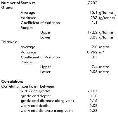
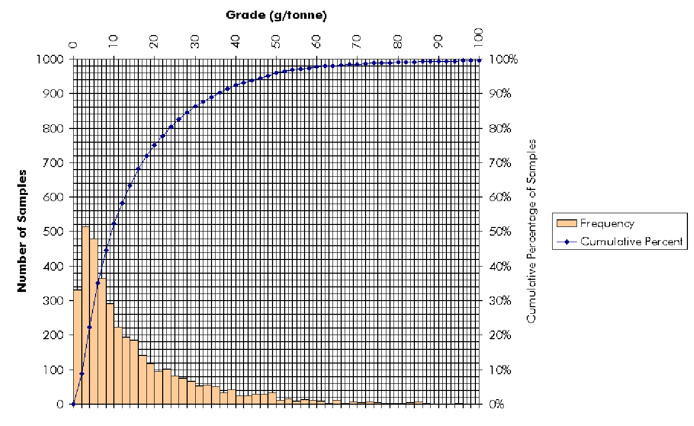
Figure 3-2: Grade histogram and cumulative distribution.
 
 
 

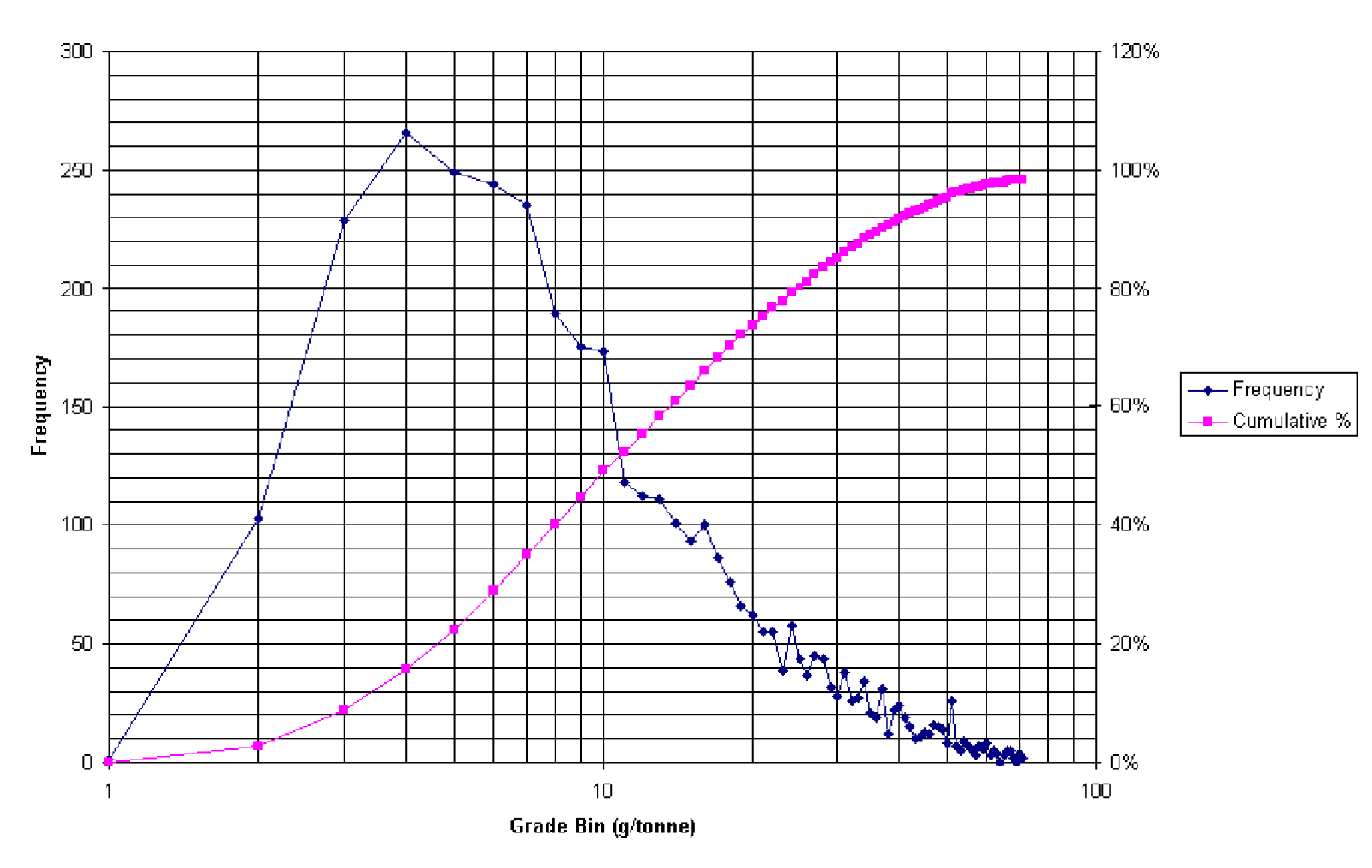
Figure 3-3: Grade histogram with cumulative distribution, plotted with a logarithmic x-axis.
 
 

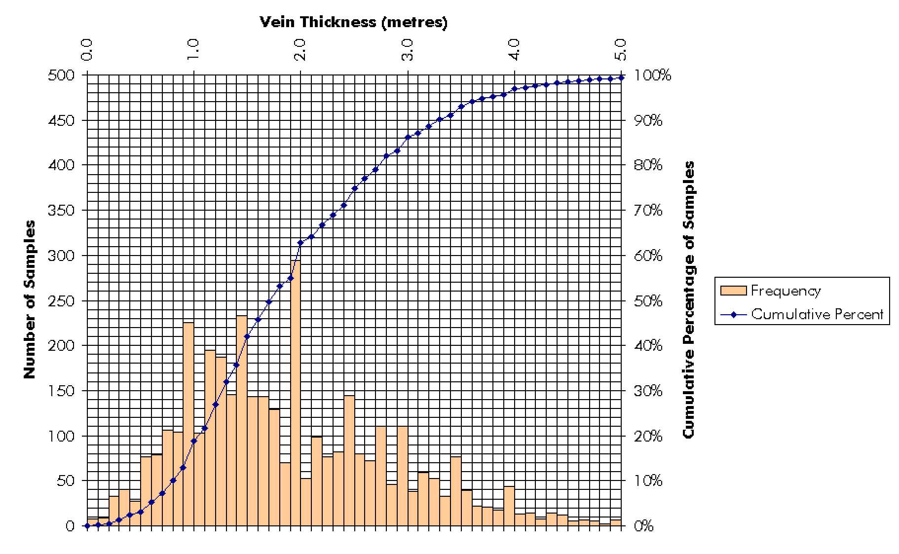
Figure 3-4: Vein thickness histogram and cumulative distribution. Notice the spikes at 1.0, 1.5, 2.0, 2.5, 3.0, 3.5, and 4.0 metres that were probably caused by measurement rounding.
 
 
 

3.3 Data Preparation
As submitted, the data was not suitable for use with geostatistics because sample coordinates had not been assigned. However, using certain reasonable assumptions, enough information was given to allow coordinates to be assigned to most samples.

The Poura mine uses a unique two-dimensional coordinate system. Distance along strike is measured in ‘profiles.’ One profile is roughly equal to the advance of a development blast. Vertical elevation is measured in ‘levels.’ Levels are named by their depth, in metres, from the collar of the main shaft. However, the elevation is not necessarily constant on a particular level.

Most of the samples are channel samples that were taken during development advances. Between each development blast, two channel samples were taken from the face. They were taken one above the other, separated by a vertical metre. Channels were chipped normal to the plane of the vein. Coordinates were not recorded for each sample. Rather, the starting and ending coordinates of a line of samples was recorded. For example, along Level 140, between Profile 20 and Profile 40, 20 samples were taken.

To assign coordinates to every sample, an X-Y coordinate system was first established for the mine. The shaft collar was given a coordinate of (1,000 metres, 1,000 metres). Using the mine’s longitudinal section in AutoCAD (Figure 3-1), the starting and ending coordinates for each line of samples was determined. A utility program was written using Microsoft QuickBASIC 4.0 to help assign coordinates to the more than 3,000 samples. Input to the program was the starting point, the ending point, and the number of samples. The program calculated a linear equation between the points and broke the line into a number of intervals equal to the number of samples. A sample coordinate was assigned at the middle of each interval.

That the samples were equally spaced along the line was an assumption, but given the circumstances, it was the most prudent assumption that could be made. Also, though two channel samples were generally taken at each new face along the development drift, there was no existing information with the samples that would enable them to be paired together. The program simplified the sampling plan by assuming a single line of samples. It output the coordinate for each sample to a file that could be imported to a spreadsheet. The full program code is given in Appendix 1.

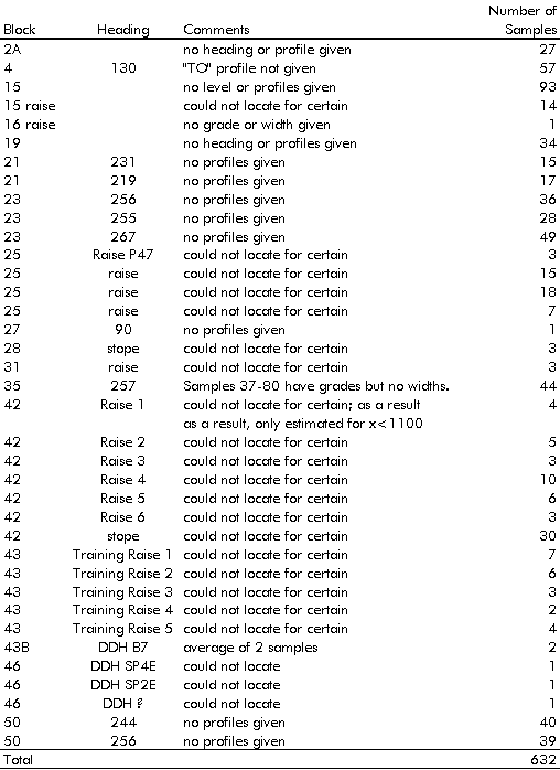
Unfortunately, not enough information was given to assign coordinates for all samples. Therefore, they were not used during kriging. Table 3-2 lists the 632 samples for which coordinates could not be assigned, as well as the reasons why.
 
 

Table 3-2: Samples for which coordinates could not be assigned.

There were also several diamond drill samples that appeared on the longitudinal section but not in the sample data set. Those samples, for which coordinates were subsequently assigned and were used during kriging, are listed in Table 3-3.
 
 

Table 3-3: Diamond drill holes that previously had not been considered and were not part of the supplied data set.

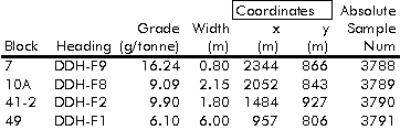
3.4 Changes
Several changes were made to make the analysis more meaningful. The first concerned the size of some of the blocks. For example, Block 22 is 790 metres long. Estimating a single grade for the entire block would not be very meaningful because a mining block is generally much smaller. Therefore, Block 22 was divided into eight separate blocks, each approximately 100 metres long. For the same reasons, Block 26 was divided roughly in half, and Blocks 40 and 41 were each divided into thirds.

Block 15 had only one sample assigned to it. Upon closer examination, it was discovered that a line of samples that had been assigned to Block 22 were taken in a line directly beneath Block 15. Those samples were subsequently used to estimate both blocks’ grades.
 

3.5 Regularization
Generally, all data must be regularized so that each sample has an identical support. Poura’s data did not require regularization because all samples were roughly equal in size and all were taken along a direction normal to the vein. When the vein is considered as a two-dimensional body, each sample appears as a point.
 

3.6 Grade and Vein Thickness Semi-variogram Modeling
MicroLYNX was used to calculate semi-variograms for grade and thickness. For each variable, variograms were calculated for four directions (+/- 22.5° ):

• 0 ° (along dip);
• 90 °(along strike);
• 45 ° (plunging south); and,
• 135 ° (plunging north).

g (h) = 0 h = 0                 (Eq. 3-1)

g (h) = C₀ + C ₁( 3h/2a – h³/2a³) h < a

g (h) = C₀ + C₁ h ³ a

where:
C(h) is the variogram value at lag h

C₀ is the nugget value

C₁ is equal to the sill value minus C₀

"a" is the range

At first glance, a logarithmic model seemed suitable for the grade data (Figure 3-6). However, a transitional linear model produced a much better fit. The equations for those lines were:
 

g (h) = 0 h = 0 (by definition)                 (Eq. 3-2)

g (h) = 3.167h + 177 0 < h £ 30

g (h) = 0.6667h + 252 30 < h £ 120

g (h) = 332 120 < h

One fact supporting the previous argument is that the semi-variogram data was poor for both the grade and the thickness data. If the poor data was the fault of, for example, assaying techniques, it would be possible to have good quality thickness semi-variogram data and poor quality grade semi-variogram data. The sample spacings were common to both variables.

Semi-variogram data that seems to exhibit "pure nugget" behaviour can be caused by a number of things. Firstly, the data could actually be "pure nugget" – the range is much smaller than the data supports (Journel and Huijbregts, 1978). When "pure nugget" is present, the fluctuations around the sill are small, which is not the case for the non-strike direction semi-variograms. Secondly, a smoothing effect could be present due to the regularization of samples. That could not be the reason because Poura samples were not regularized. Thirdly, the poor semi-variograms could be caused by a fluctuation effect – too few data used for the semi-variogram construction. That was most likely the cause of the poor non-strike direction semi-variograms.

The semi-variograms show that the thickness is less variable than the grade. The thickness semi-variogram has a sill of 0.60 m². The sill is also known as the a priori variance. That corresponds to a standard deviation of 0.77 m. The grade semi-variogram has a sill of 332 (g/tonne)², equivalent to a standard deviation of 18.2 g/tonne. To compare the two variables, the thickness standard deviation was multiplied by the ratio of the grade’s arithmetic mean to the thickness’ arithmetic mean:

Normalised Thickness Standard Deviation = 0.77 m x 15.1 g/tonne

2.0 m

= 5.8 g/tonne

Since 5.8 g/tonne is much less than the grade’s standard deviation of 18.2 g/tonne, vein thickness is less variable than grade.

For reasons that were described in Section 2.7, the semi-variograms that were calculated from the sample supports g_v*(h) can be treated as if it were an estimator of the point semi-variogram model g (h).
 

Table 3-4: Number of sample pairs for each lag interval for the four principal directions.

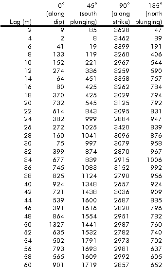
Figure 3-5: Vein thickness semi-variogram experimental data and fitted spherical model for search azimuth 90° +/-22.5° (along strike).
 
 

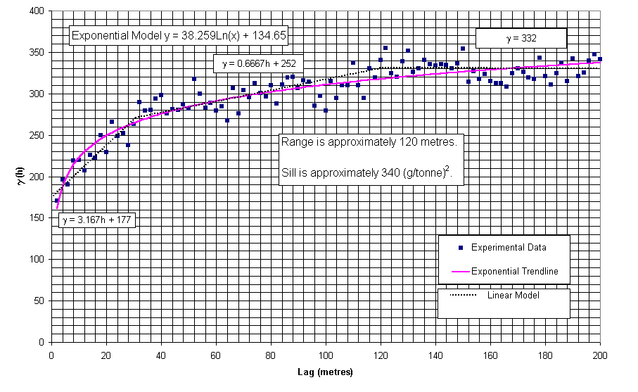
Figure 3-6: Grade semi-variogram data and fitted models for search azimuth 90° +/- 22.5° (along strike). The transitional linear model fits the experimental data much more accurately than the exponential model.
 
 

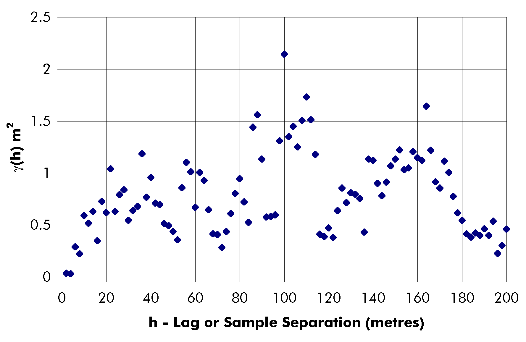
Figure 3-7: Vein thickness semi-variogram data for search azimuth 0° +/- 22.5° (along dip). No model could be fitted to the erratic experimental data.
 
 

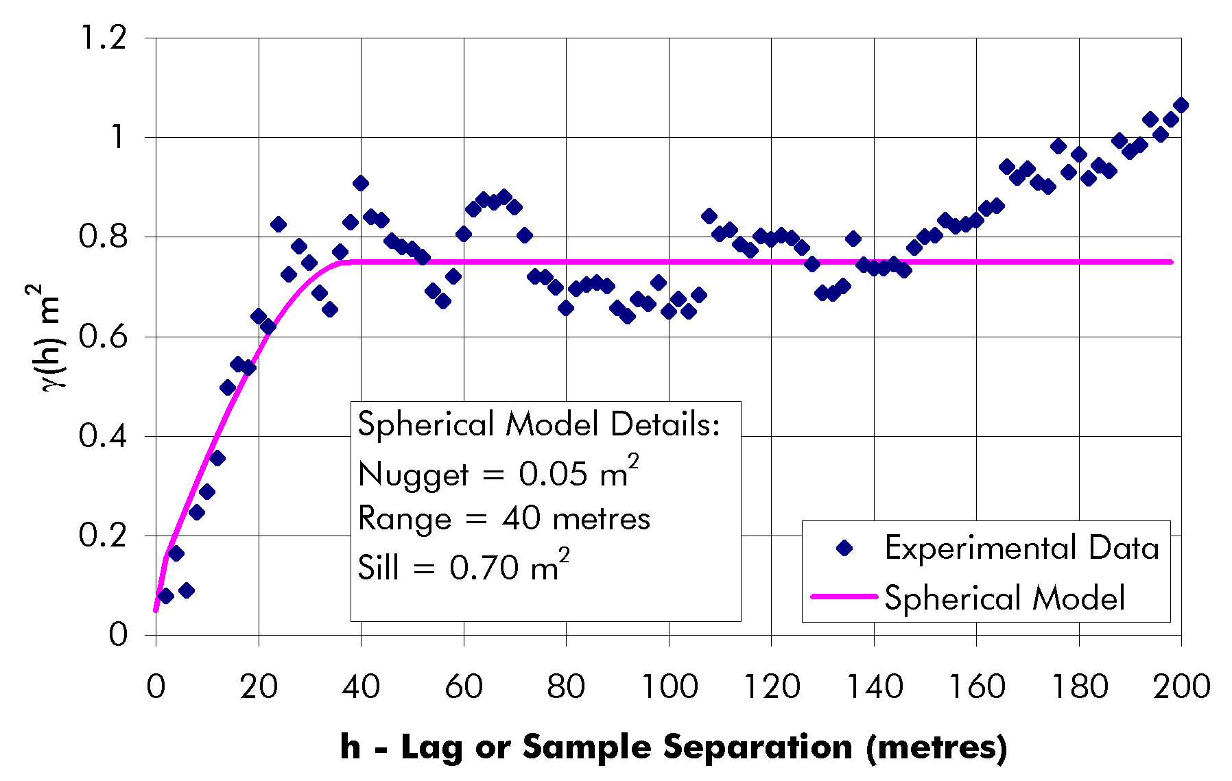
Figure 3-8: Vein thickness semi-variogram data for search azimuth 45° +/- 22.5° (south plunging). Though the experimental data was more erratic than the along-strike data, a spherical model was fitted that had parameters (nugget, range, and sill) similar to the along-strike model.
 
 
 
 

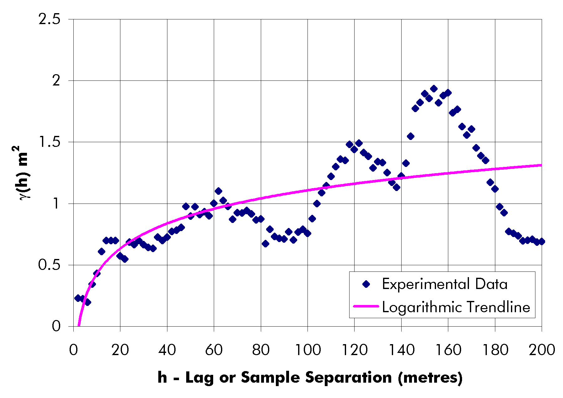
Figure 3-9: Vein thickness semi-variogram data for search azimuth 135° +/- 22.5° (north plunging). An exponential model was tentatively fitted, but it would not be prudent to use it because the data is so erratic compared to the along-strike experimental data.
 
 

Figure 3-10: Grade semi-variogram data for search azimuth 0° +/- 22.5° (along dip). No model could be fitted to the erratic experimental data.
 
 
 
 

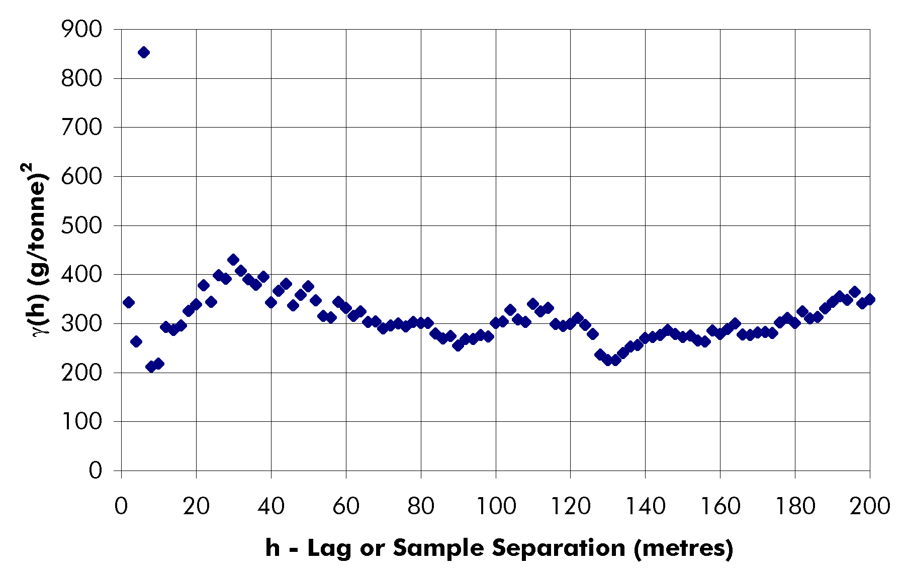
Figure 3-11: Grade semi-variogram data for search azimuth 45° +/- 22.5° (south plunging). Again, no model could be fitted to the experimental data.
 
 
 
 

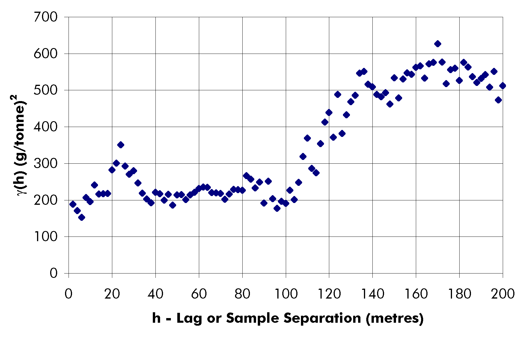
Figure 3-12: Grade semi-variogram data for search azimuth 135° +/- 22.5° (north plunging). No useful or realistic model could be fitted to the experimental data.
 
 
 
 

4. Development of Kriging Methodology

Another major reason why ordinary block kriging is sometimes not used is because it sometimes overestimates the grade of deposits with skewed distributions (see Section 1.7). However, in a case reported by Deutsh (1989) where the ordinary kriging overestimated the grade by about twenty-five percent, the raw semi-variogram data was so noisy that no trend could be discerned. That is not the case for Poura’s grade and thickness semi-variograms.

Poura’s grade distribution is skewed (see Section 3.2). However, the coefficient of variation of the grade data is only 1.1 (0.5 for vein thickness data) (see Section 3.2). According to Dominy et al (1997) and Fytas et al (1990), ordinary block kriging performs well when the coefficient of variation is close to (or less than) one.

For the reasons described above, it was decided to use ordinary block kriging as a first pass at estimating Poura’s resources. If, after production begins and the true block grades can be determined, the grade is shown to have been overestimated, another kriging method such as indicator kriging can be explored.

In all of the cases that were reviewed, the evaluators used rectangular blocks of uniform size. An instance could not be found in the literature where an evaluator used oddly shaped blocks during ordinary block kriging. Poura’s remnant blocks and pillars are oddly shaped and cannot be accurately represented on a regular grid. The general practice when one is faced with an oddly shaped block is to estimate the grade and variance of regular blocks within the oddly-shaped block, then combine the estimates to give a single grade and variance (Journel and Huijbregts, 1978). That process becomes complicated when the same sample group is used to estimate each smaller block. Therefore, rather than take that route, it was decided to develop and use a method whereby an oddly shaped block could be kriged all at once using ordinary block kriging.
 

4.2 Krige2D
Throughout its relatively short life, geostatistics has been widely criticised as being a black box approach to resource estimation. Geostatistical computer packages are widely available. With no knowledge of geostatistics, a user can carry out a ‘geostatistical’ resource estimate for a deposit. Like any other method, geostatistics, when improperly applied, can produce erroneous results that the user may or may not notice.

MicroLYNX ’98 is an Australian mine planning computer program that includes geostatistical functions. Semi-variograms can be calculated and point or block grades can be calculated using kriging. Such a package is a useful tool; however, the methods are not thoroughly explained in the program documentation. There are dozens of different kriging methods, but MicroLYNX simply refers to its methods as ‘kriging.’

To avoid taking a ‘black box’ approach to estimating Poura’s resources, the author wrote a block kriging computer program called Krige2D using the Microsoft QuickBasic 4.0 programming language. A benefit of Krige2D is that a single estimated grade and variance can be calculated for an odd shaped block of any size. Many commercially available geostatistical packages, including MicroLYNX, can only handle blocks of uniform size and shape.

Each term in the -matrix (Section 2.8) is the covariance between a sample and the stope area. Ideally, it is calculated by integrating the covariance over the stope area. Practically, Krige2D performs the integration arithmetically using the block’s internal points.

In Krige2D, each block is considered sequentially. Krige2D lays a mesh of internal points over the block using the block boundary equations that are input through the file StopeInp (Appendix 4). For each block, StopeInp contains linear equations that describe its upper and lower boundaries. Within a given range in x, each equation’s slope and y-intercept are included.

In calculating internal point coordinates, Krige2D starts at the first lower boundary and works its way up to the first upper boundary. It then moves one unit in the positive-x direction and determines if the upper and lower boundary equations are still appropriate – ie, if their x-limits were not passed. If one or both x-limits were passed, Krige2D uses the next boundary equation. For reasons that will be described later, a one metre spacing was used for the analysis.

Krige2D reads the block’s samples from the input file SampInp (Appendix 4) and calculates the -matrix (covariance between samples). Each block has a different -matrix because different samples are used for each block. Both grade and thickness semi-variograms are shown; however, only the appropriate one is used while the other is ‘commented-out’. The subroutine Dgselu is used to find the LU decomposition of the -matrix. After the -matrix (average covariance between each sample and the internal points) is calculated, the LU decomposition is used in the subroutine Dnslov to solve the kriging equations for the sample weights.

Solving the system of kriging equations was accomplished using two functions, Dgselu and Dnsolv, that were provided by Dr. Gordon Fenton, a professor at Dalhousie University. The functions were written in Fortran, so they required conversion to QuickBASIC.

The estimated mean grade is calculated using the sample weights. To calculate the estimated variance, the block covariance is calculated in the BlockCov subroutine. In that subroutine, the average covariance between unique pairs of internal grid points is calculated. As an example of BlockCov’s methodology, consider a set of n internal points. The covariance between each pair of internal points could be expressed as an (n x n) matrix. The values on the diagonal (1,1; 2,2; 3,3; etc) are not unique because any point and itself does not constitute a pair. Also, only the pairs above or below the diagonal, but not both are considered because, for example points 1,2 and 2,1 are the same pair – they are not unique. The covariances between unique pairs are averaged to give the block covariance.

The weighted covariance is also needed to determine variance. It is calculated in the main module by summing the product of each sample’s weight and the average covariance between the sample and the area (its -matrix value). The variance is then calculated using the equation:
 

Estimated Variance = Block Covariance – Weighted Covariance + Lagrange value

Krige2D produces a number of output files. One output file named Output contains the details of the matrix calculations. That file was used to verify Krige2D’s accuracy in Section 4.3. Another file named OutSumm is a summary of the kriging results. The four OutSumm files, for grade and thickness at one and two metre spacings, are shown in Appendix 5. A third file, named IntPtOut, contained the coordinates of the blocks’ internal points. As a check, they were laid over the longitudinal section (Figure 1-2) to ensure they were within the block boundaries.
 

4.3 Verifying Krige2D
To verify Krige2D’s results, a simplified kriging arrangement was designed that consisted of two stopes (Figure 4-1). One stope is rectangular while the other is oddly shaped. The stope boundaries, sample coordinates, and sample values were input to Krige2D. To simplify the process, sample coordinates and values were identical for each stope. Only the stope boundaries were different. For calculating the -matrix (Section 2.8), Stopes 1 and 2 were broken up into four and three equal parts, respectively. A simple correlation function was assumed. Krige2D estimated Stope 1’s grade as 15.23 g/tonne and its variance as 9.13 (g/tonne)². It estimated Stope 2’s grade as 14.29 g/tonne and its variance as 3.27 (g/tonne)². To compare, grade and variance were calculated manually, in a spreadsheet, using the same parameters. Both methods gave identical results, indicating that Krige2D can accurately carry out block kriging calculations. Details of the program verification are given in Appendix 3.
 

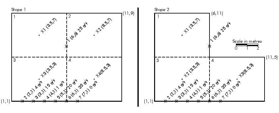
Figure 4-1: Test stopes for confirming Krige2D's results.
 
 

4.4 Krige2D Input
The kriging matrices made use of the covariance function C(h) rather than the semi-variogram function g (h). Making use of the relationship between the two functions that was described in Section 2.3, the following set of grade semi-variograms were input to Krige2D:
 

C(h) = 332 h = 0                 (Eq. 4-1)

C(h) = 155 – 3.167h 0 < h £ 30

C(h) = 80 – 0.6667h 30 < h £ 120

C(h) = 0 h < 120

The thickness structure was input as:
 

C(h) = 0.82 h = 0                 (Eq. 4-2)

C(h) = 0.6 – 0.6( 3h/110 – h³/332750 ) 0 < h £ 55

C(h) = 0 h < 55

4.5 Observations
Several observations were made as kriging was being carried out.

4.5.1 Point Spacing
An internal point spacing of two metres is the greatest spacing that could be used for the Poura blocks because parts of some of the blocks are only about two metres wide. For example, Block 22 is a long horizontal sliver with dimensions of about eight hundred metres long by less than four metres tall. As one can see in Figure 4-2, an internal point spacing of two metres yields points that are not very evenly spaced with respect to the block boundaries. The upper points are closer to the boundary than the lower points.

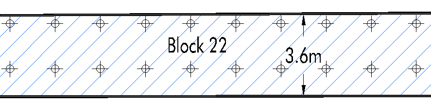
Figure 4-2: A portion of Block 22 showing the block kriging internal grid points (shown here with a two metre spacing).
 
 

Kriging was first carried out using an internal spacing of two metres. The complete results are shown in Appendix 5. However, an erroneous result was noted for one of the blocks. Block 7’s estimated thickness variance was calculated as -0.000914 m². That result is mathematically impossible because variance is equal to the square of standard deviation. The error was investigated, but no cause could be discovered; however, the coarse sample spacing was suspected as the cause of the error.

Ideally, as described in Section 2.9, the -matrix should be calculated by integrating the covariance over the block area. Practically, a grid of internal points is used to approximate integration. The finer the grid spacing, the closer the grid comes to integration. Block 7 is shown in Figure 4-3 with a two metre grid spacing. One can see that a two metre spacing seems too coarse for Block 7. One can also surmise that such a grid would do a poor job at approximating integration.
 
 

Figure 4-3: Block 7 showing internal points at a two metre spacing.
 
 

Therefore, to explore the theory that a two metre point spacing was too coarse, it was decided to try kriging using an internal point spacing of one metre. A one metre spacing yields an internal point grid that is more evenly spaced throughout the blocks. From a mathematical standpoint, it also yields a more accurate answer because the finer the internal point spacing, the closer Krige2D approximates integration.

Kriging using a one metre spacing produced no erroneous results (Appendix 5). The estimated mean grades and thicknesses were negligibly different for the two different internal point spacings. Neither spacing produced consistently higher or lower results. There was also virtually no difference between the grade variances. Apart from producing an erroneous variance for Block 7, kriging using a two metre spacing produced quite similar results as using a one metre spacing.

The complete results can be seen in Appendix 5. Output summary files are shown for grade and thickness at one metre and two metre spacings. The estimated grade accumulation (estimated grade x estimated thickness) for each block is presented graphically in Figure 5-1. A summary of results is presented in Table 5-1. Detailed results are given in Table 5-2. All grades are reported as undiluted grades. 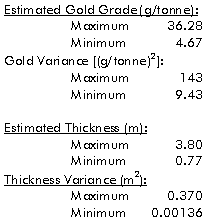The estimated mean grade ranged between 4.67 g/tonne (Block 24) and 36.28 g/tonne (Block 40-3) (Table 5-1). Grade variance ranged between 9.43 (g/tonne)² (Block 10A) and 143.3 (g/tonne)² (Block 40-3). Estimated thickness ranged from 0.77 metres (Block 40-2) to 3.81 metres (Block 54). Thickness variance ranged between 0.00136 m² (Block 7) and 0.370 m² (Block 40-3).
 
 

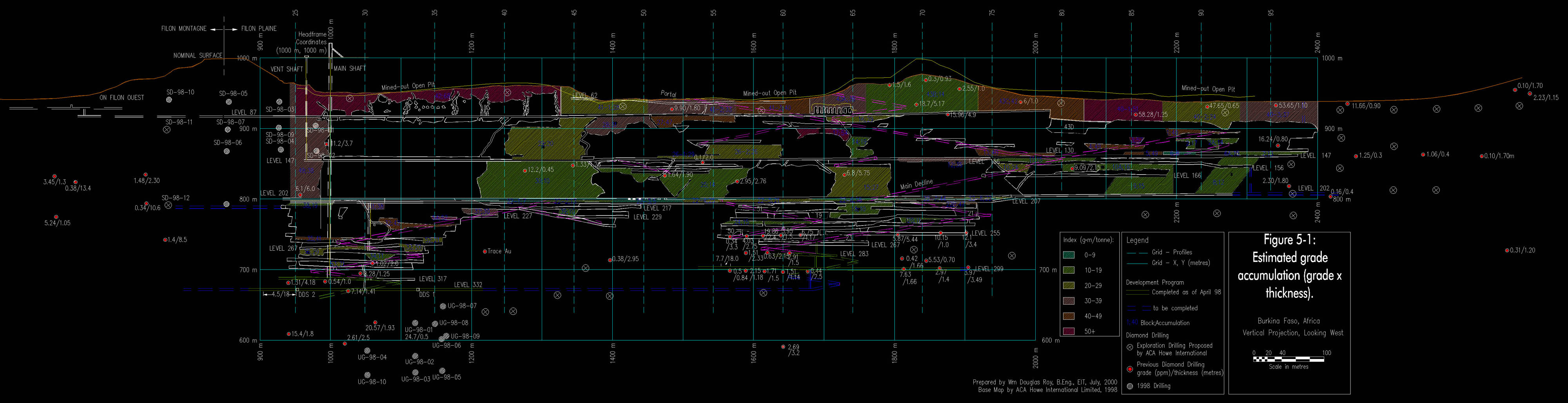
Figure 5-1: Estimated grade accumulation (grade x thickness).
 
 
 
 

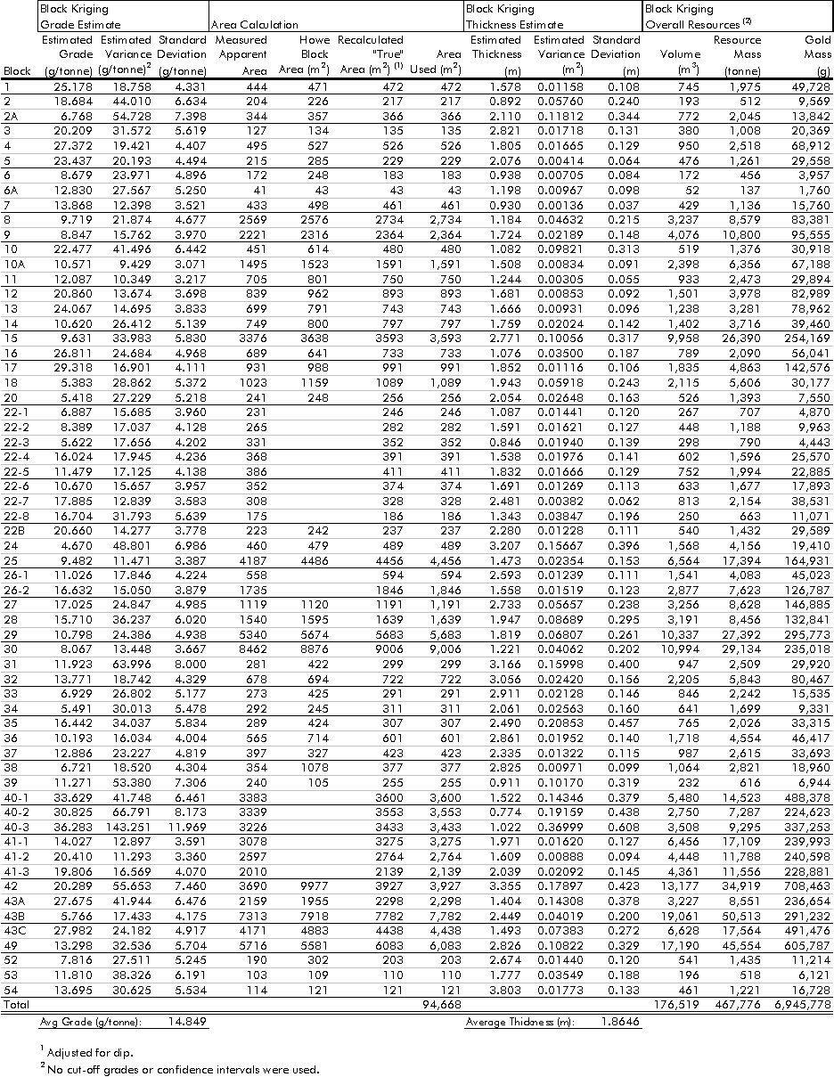
Table 5-1: Summary statistics of kriging results.

The average (volume-weighted) mean grade was calculated as 14.85 g/tonne (Table 5-2). The average (volume-weighted) mean block thickness was calculated as 1.86 metres. Resources were calculated using each block’s estimated mean grade and thickness. A block’s estimated mean is the expected value. Statistically, it is the most likely value, where an actual outcome is equally likely to be higher or lower.

Expected volume was calculated by multiplying each block’s thickness by its area. Each block’s mass was calculated using the estimated specific gravity of 2.65 (Titaro and Hannon, 1998). The total gold mass in each block was determined by multiplying its expected grade by its mass. Then, a grade-tonnage curve was constructed that plotted the resource’s mass and average grade against cut-off grade.
 
 
 

Table 5-2: Overall kriging resources (variances not considered).

 
 
 
 

The grade-tonnage curve is very informative, widely used, and well accepted by the mineral industry. Its construction is simple: at each cut-off grade on the x-axis, determine the block grades that exceed the cut-off. Sum the mass and gold mass of those blocks and calculate an average grade.
 
 

5.1 Using Confidence Limits in Risk Analysis
Most resource estimates do not make use of geostatistics. Each block’s actual mass and grade are both equally likely to be higher or lower than the expected values. Using conventional methods, it is impossible to describe the spread, quantified by the variance or standard deviation, of the distribution. Therefore, there is a great deal of uncertainty inherent to non-geostatistical estimating methods.

Using geostatistics, the estimated variance is calculated along with the estimated mean. Because the variances of each block’s grade and thickness are known, the confidence of the estimate can be explored. It is already known that the grade, for example, is equally likely to be higher or lower than the estimated mean. That equates to 50 % confidence that the actual grade will be higher than the mean grade. Most people in industry are not satisfied in being only fifty percent confident in an estimate. A mine operator wants to know the grade with more certainty; for example, (s)he prefers to know, with seventy-five percent confidence, that the actual grade will be higher than a chosen value.

To determine that grade, one must first know the grade’s distribution type. The distribution that is most often used is the normal or Gaussian distribution because it is the most often seen in mining practice (Journel and Huijbregts, 1978).

In most areas of science, confidence limits are calculated by centering the desired confidence or probability over the mean value. In most cases, the confidence limit is bounded by two values – one lower, one higher than the mean. Figure 5-2 shows an example (normal) probability distribution with a mean of 20 g/tonne and a standard deviation of 5 g/tonne. In that example, there is a confidence (probability) of fifty percent that the actual value will be between 16.6 g/tonne and 23.4 g/tonne.

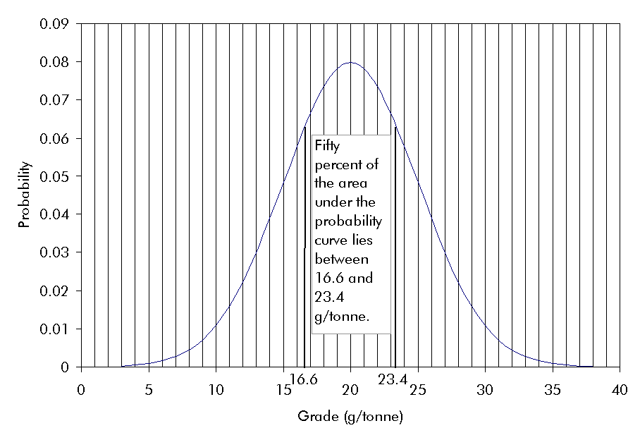
Figure 5-2: Probability plot for a mean grade of 20 g/tonne and a standard deviation of 5 g/tonne. Fifty percent of the area under the curve is between 16.6 and 23.4 g/tonne.
 
 

However, in mining applications, it is not desirable to use an upper limit for the actual grade. We would be perfectly content if the actual grade were higher than 23.4 g/tonne (Figure 5-2). Indeed, we wish that the actual grade were high as possible. For mining, it is more desirable to know, with a certain confidence (probability), the lowest possible value for the actual grade.

For example, in an economic analysis, it is desired to know the grade for which there is a seventy percent chance that the actual grade will be greater (Figure 5-3). That grade corresponds to 17.4 g/tonne. In other words, there is only a thirty percent probability that the actual grade will be less than 17.4 g/tonne.

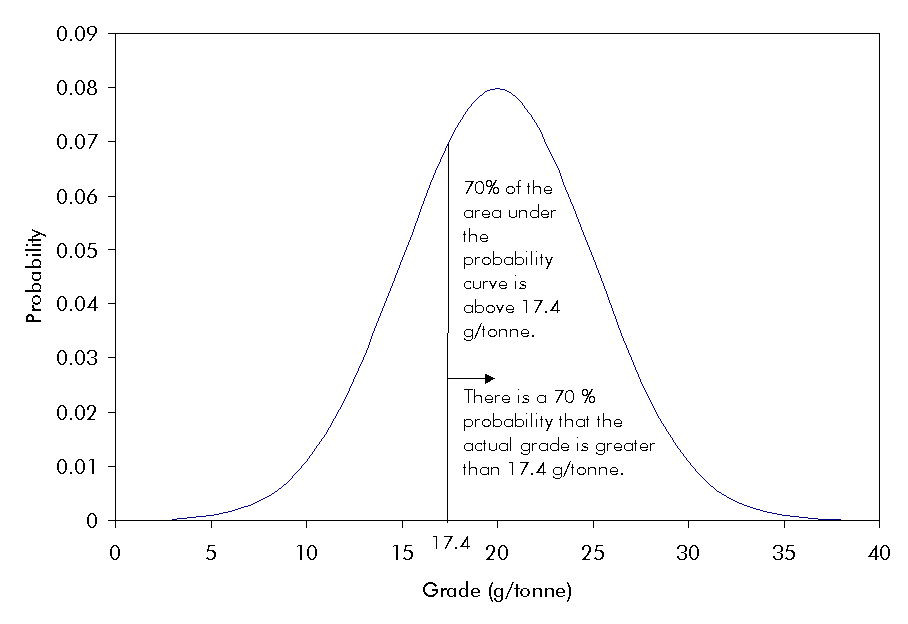
Figure 5-3: Probability plot for a mean grade of 20 g/tonne and a standard deviation of 5 g/tonne. Seventy percent of the area under the curve is above 17.4 g/tonne.
 
 

The grade-tonnage curve is an effective tool for managing risk. We have already discussed the construction method for the expected or most likely values. Using the variances of each block’s grade and thickness, a whole suite of grade-tonnage curves can be constructed – one for each confidence level. For example, an operator wishes to be seventy percent confident that the actual block grade will be higher than a chosen value (cut-off grade). To calculate a grade-tonnage curve based on that lower confidence limit, a certain cut-off grade is first considered. For each block, using the estimated mean grade and variance (the block’s grade distribution), the grade is calculated for which there is a seventy percent probability that the actual grade is greater.

If that calculated grade (17.4 g/tonne in Figure 5-3) is greater than the particular cut-off grade under consideration, the block is included in the resources for that cut-off. After a block has been included, its mass is calculated using the thickness for which there is a seventy percent chance that the actual thickness will be greater. Every block is considered in the same manner.

The mass and gold mass of each block above cut-off is summed and the average grade is calculated. The grade-tonnage curve is constructed by plotting the resource mass above cut-off versus each cut-off grade. The average grade of the resource above cut-off is also plotted.

The process is repeated for a range of desired confidences. For example, separate grade-tonnage curves are calculated for 40 %, 60 %, 70 %, 80 %, and 90 % confidences. The result is a family of grade-tonnage curves. That allows the end-user to consider different scenarios when carrying out an economic analysis. For example, one economic analysis could be carried out using a 70 % confidence. The intersection of the cut-off grade (known) on the x-axis and the 70 % confidence grade-tonnage curve reveals the mass of the resource. The average grade of that resource is shown by the intersection of the cut-off grade (x-axis) and the ‘average grade at 70 % confidence’ curve. The economic analysis would be carried out using that mass and average grade, the result being various economic indicators such as net present value and internal rate of return. To explore the project’s sensitivity, the whole process could be repeated using other confidence limits.
 

5.2 Kriging Resources (no Cut-off Grade Considered)
Undiluted kriging resources were calculated using the estimated mean grade, estimated mean thickness, and block area. These ‘overall’ resources did not consider the variances of each estimate. When no cut-off grade is considered, resources consist of 468,000 tonnes with an average grade of 14.85 g/tonne. The resource contains 6,946,000 grams (223,000 toz) of gold. The average vein thickness was 1.86 metres. Cut-off grades are considered in Section 5.4. In that section, these ‘overall’ resources correspond to a lower confidence limit of 50 % (Table 5-4). It must be noted that these resources cannot be compared directly to those estimated by ACA Howe in 1998. A proper resource comparison is made in Section 5.3.
 

5.3 Comparison Between Kriging Resources and ACA Howe’s Resources
ACA Howe calculated block grade and thickness using an arithmetic method. For each block, each sample grade was cut to 57.0 g/tonne. Each cut grade was then multiplied by the vein thickness. Those values were summed and divided by the arithmetic average thickness to give the ‘average cut grade.’ Another block grade was calculated by calculating the natural logarithm of each thickness-weighted grade. Those values were summed and the anti-log of the sum was calculated. That value was divided by the arithmetic average thickness to give the ‘log average cut grade.’ The estimated block grade was finally calculated by averaging the ‘average cut grade’ and the ‘log average cut grade.’ ACA Howe adopted such a complicated procedure for estimating the grade because from past experience, the ‘average cut grade’ overestimated the block grades while the ‘log average cut grade’ underestimated the block grades.

The ‘overall’ undiluted kriging resources (Section 5.2) were compared with ACA Howe’s undiluted resources (Table 5-3). Comparing them generally, the average grade for the block kriging resource was 14.85 g/tonne - 2.5 g/tonne higher than ACA Howe’s arithmetic average grade of 12.34 g/tonne. The average thickness was essentially equal for both estimates at 1.86 metres and 1.84 metres for the block kriging and arithmetic methods, respectively. The arithmetic method estimated that the grade and, to a lesser extent, the thickness were lower.

A more detailed comparison was also carried out on selected blocks. No cut-off grade was used for the comparison. The blocks that were included were those for which the same samples were used in each method. In all, 50 of the 62 blocks were compared. In the blocks that were compared, ACA Howe’s arithmetic method estimated that the resources were larger by 6,400 tonnes. However, the arithmetic method estimated much less gold in the resource. Block kriging estimated that there were 1.2 million more grams of gold in the blocks that were compared. Assuming a gold price of $US 300 per troy ounce ($CA 14.10 per gram), 1.2 million grams of gold is worth $CA 17 million.
 
 
 

Table 5-3: Comparison between kriging resources and those that were estimated by ACA Howe.

 
 

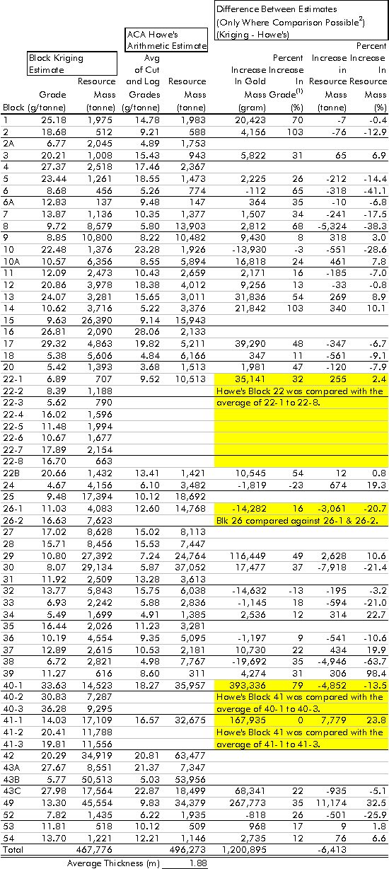
5.4 Cut-off Grades
Cut-off grades were considered by calculating grade-tonnage curves (see Section 5.0 for more information). One grade-tonnage curve, showing resources above cut-off and average grade versus cut-off grade, was calculated for several lower limits of confidence: 40 %, 50 %, 60 %, 70 %, 80 %, and 90 %. The data that was used to construct the 50 % grade-tonnage curve (Figure 5-4) is shown in Table 5-4. The data sets used to construct the other curves are given in Appendix 6.
 
 

Table 5-4: Resources considering cut-off grades and confidence in grade and vein thickness using a 50 % lower limit of confidence.

 
 
 

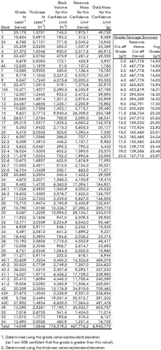
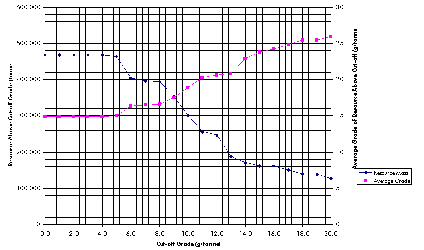
Figure 5-4: Grade-tonnage curve showing resource quantity and average grade using a 50 % lower limit of confidence.
 
 

Figure 5-5 shows all of the grade-tonnage curves in a single chart. Generally, as do all grade-tonnage curves, as the cut-off grade increases, the undiluted resource above cut-off decreases and the average grade increases. At the lower confidence limits such as 40 % confidence, the quantity and average grade remain stable until the 6.0 g/tonne cut-off grade is reached. Only after 6.0 g/tonne do the quantity start decreasing and the average grade start increasing. However, at higher confidence limits such as 90 %, the quantity decreases as soon as the cut-off grade rises above zero. The average grade begins increasing at the same point. In other words, at a low confidence limit such as 40 %, all of the blocks’ grades are above cut-off until a 6.0 g/tonne cut-off grade is reached. However, at high a high confidence limit such as 90 %, some of the blocks’ grades are lower than even the 1.0 g/tonne cut-off.

An interesting, though erroneous aspect of using confidence limits to construct grade-tonnage curves is that it is mathematically, though not practically possible to have a block grade or thickness that is less than zero. For example, Block 2A has an estimated mean grade of 6.77 g/tonne with a standard deviation of 7.40 g/tonne (Table 5-2). At a 90 % lower limit of confidence, Block 2A’s minimum grade is -2.71 g/tonne (Appendix 6). Because is not possible in nature to have a negative concentration of anything, any negative concentrations were changed to zero.

A mine operator would want to be at least 60-70 % confident in the grade and quantity of the resource. Recall that ACA Howe’s estimate would be equivalent to the 50 % confidence limit (expected value). It can be seen in Figure 5-5 that when no cut-off grade is considered, the resource drops from 468,000 tonnes to 435,000 tonnes (a 7 % decrease) when the confidence is increased from 50 % to 70 %. The average grade decreases from 14.85 g/tonne to 11.94 g/tonne (a 20 % decrease). However, ACA Howe used 5.0 g/tonne as the cut-off grade in their feasibility study. At that cut-off grade, the resource drops from 464,000 tonnes to 367,000 tonnes (a 21 % decrease) when the confidence is increased from 50 % to 70 %. The average grade decreases from 14.94 g/tonne to 13.55 g/tonne (a 9 % decrease).

A confidence of one standard deviation is often quoted in trade magazines. That corresponds to 84 % confidence. At a 5.0 g/tonne cut-off grade, the resource drops from 464,000 tonnes to 278,000 tonnes (a 40 % decrease) when the confidence is increased from 50 % to 84 % (Figure 5-6). The average grade decreases from 14.94 g/tonne to 12.46 g/tonne (a 17 % decrease).
 

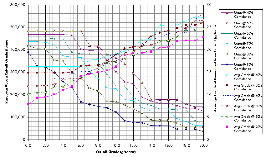
Figure 5-5: Grade-tonnage curve showing resource quantity and average grade using several lower limits of confidence.
 
 

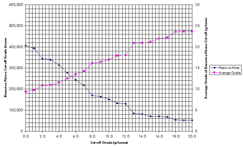
Figure 5-6: Grade-tonnage curve showing resource quantity and average grade using a lower limit of confidence equal to 84 %.
 
 

5.5 Comparing Geostatistical and Non-geostatistical Methods
Geostatistics is the only resource estimating method that yields not only the estimated mean grade, but also the estimated variance or spread of the grade distribution. Other estimating methods, such as inverse distance weighting and graphical methods such as the polygonal method or triangular method, yield only the estimated grade with no indication of the distribution variance. Without the variance, a risk analysis of the resource estimate cannot be carried out. Economic risk is described further in Sections 6.2.1 and 6.2.2.
 

5.6 Exploration Potential
Figure 5-1 shows the grade accumulation (grade x vein thickness) for each block. Analysing the grade accumulation is a good method for predicting trends in mineralisation. It is difficult to evaluate the resources of a vein deposit such as this one using the results of diamond drilling or chip sampling. Individual samples, even groups of samples, do not provide a clear picture. From Figure 5-1, it can be seen that the accumulation is consistently the highest around the ends of the current mine workings. Specifically, south of Profile 30 on the local grid or 1,250 metres on the new grid, both along strike and down dip, the accumulation is consistently higher than twenty gram× metres per tonne. Similarly, at the northern end of the workings around Block 40, the accumulation is around fifty gram× metres per tonne.

The best exploration targets would be along strike in both directions from the current workings. Second best would be down dip from the southern end of the current workings. Because, by itself, diamond drilling is inadequate for properly evaluating those areas, it should be supplemented by driving exploration drifts and raises. The vein material removed can be processed as a bulk sample. Also, chip sampling should be carried out with a one or two metre spacing.

Near the bottom of the current workings, north of Profile 30 is excellent lower-grade material with a grade accumulation of more than ten gram× metres per tonne. With a lower priority, down-dip of the area should be explored in the same manner.
 
 
 

6. Conclusions and Recommendations

1. A statistical analysis was carried out on the 3,232 samples that were used in the analysis. The average grade was 15.1 g/tonne with a variance of 283 (g/tonne)². The average thickness was 2.0 metres with a variance of 0.992 m².
2. The computer program Krige2D that was written by the author for this investigation can reliably calculate a block’s estimated grade and variance using ordinary block kriging. Krige2D is unique in that a single estimated grade and variance can be estimated for an oddly shaped block of any size.
3. The raw semi-variogram data followed a clear path to which models could readily be fit. The grade semi-variogram was isotropic and was discovered to follow the following transitional linear model:

 
g (h) = 0 h = 0 (by definition)

g (h) = 3.167h + 177 0 < h £ 30

g (h) = 0.6667h + 252 30 < h £ 120

g (h) = 332 120 < h
 

4. The vein thickness semi-variogram was also isotropic and could be described by a spherical model with a range of 55 metres, a sill of 0.60 m², and a nugget value of 0.22 m².
5. Block kriging using an internal point spacing of two metres produced an erroneous result. Using a one metre spacing produced no erroneous results.
6. The blocks’ areas were re-calculated and many of them were different than those that were reported by ACA Howe.
7. Estimated grades and variances were calculated for each block using block kriging. The estimated undiluted mean grade ranged between 4.67 g/tonne (Block 24) and 36.28 g/tonne (Block 40-3). Grade variance ranged between 9.43 (g/tonne)² (Block 10A) and 143.25 (g/tonne)² (Block 40-3). Estimated thickness ranged from 0.774 metres (Block 40-2) to 3.808 metres (Block 54). Thickness variance ranged between 0.00136 m² (Block 7) and 0.36999 m² (Block 40-3).
8. The mean grade was used to calculate ‘overall’ undiluted resources for the remnant blocks. When no cut-off grade is considered, resources consist of 468,000 tonnes with an average grade of 14.85 g/tonne. The resource contains a total of 6,946,000 grams (223,000 troy ounces) of gold and has an average vein thickness of 1.86 metres.
9. Block kriging estimated the average grade to be 2.51 g/tonne higher than ACA Howe’s estimate of 12.34 g/tonne. There was very little difference between the estimated vein thicknesses. When the blocks for which the same samples were used in both estimates were considered, it was found that block kriging estimated the quantity of gold to be 1.2 tonnes higher.
10. Using the estimated mean grades and thicknesses with a 50 % lower confidence limit and a cut-off grade of 5.0 g/tonne, the undiluted resource consists of 464,000 tonnes with an average grade of 14.94 g/tonne.
11. Using the estimation variances for grade and thickness, a process was developed for exploring how confidence affects a deposit’s resources. Grade-tonnage curves, indexed by lower confidence limits, were developed using grade and vein thickness variances.
12. When confidence in the estimate was considered, the undiluted resource falls from 464,000 tonnes to 367,000 tonnes (a 21 % decrease) when the confidence increases from 50 % (mean value) to 70 %. The average grade decreases from 14.94 g/tonne to 13.55 g/tonne (a 9 % decrease).

6.2 Recommendations for Future Work

• An economic analysis should be carried out (See Sections 6.2.1 and 6.2.2). The products of that analysis should include a table of confidence versus net present value, as well as the project’s expected profit. If the results of that economic analysis are positive, Sahelian International Goldfields should begin mining the deposit.
• Block kriging should be used with the above economic analysis to optimise the sample spacing of future exploration programs.
• Exploration should be carried out in the following locations, from highest to lowest priority:
• along strike from the current workings in both directions;
• down dip from the southern part of the workings (ie: south of Profile 30 on the local grid or 1,250 metres on the new grid); and,
• down dip from the northern part of the workings (ie: north of Profile 30);
Exploration should consist of diamond drilling supplemented with drifting and raising within the vein to collect bulk samples. The openings should also be chip sampled using a one or two metre spacing.

6.2.1 Using Confidence Limits in Making a Production Decision
Confidence limits can be used when making a production decision. However, a model of the project’s after-tax cash flow is required, which was beyond the scope of this investigation. If such an economic model were constructed, it would be best to consider all of the remnant ore blocks. This investigation considered only a portion of them.

The best method of determining which confidence limit to choose is through an economic analysis. The expected after-tax cash flow is modeled based on a confidence limit of 50 %. Using the 50 % confidence grade-tonnage curve, one can extract the mass above cut-off and its average grade. Those values define the resource base for the cash flow. The process is repeated for all other confidence limits – 40 %, 60 %, 70 %, 80 %, and 90 %. While carrying out the analysis, one must keep in mind that as the confidence level increases, the resource base decreases in quantity. As the resources decrease, the capital costs generally decrease and the operating costs increase. A change in mining method may even be necessary. At the end of the analysis, the various profitability indicators such as net present value, internal rate of return, payback period, etc will be defined for each confidence limit. Table 6-1 is a fictional example of the results of such an analysis.
 

Table 6-1: Fictional example of the results of a profitability analysis using confidence limits.

Confidence Limit (%)	Net Present Value of Operation Using A 20 % Discount Rate (Millions of Dollars)
40	10.4
50	6.0
60	2.9
70	-1.1
80	-4.1
90	-8.7

The next step is to review the results and decide whether the operation is profitable enough for the level of risk involved. Characteristically, the higher the confidence limit, the less profitable the operation will be. As in Table 6-1, an operation might have a positive net present value (NPV) up to a confidence limit of 60 %. However, it might have a negative NPV at and above a confidence limit of 70 %. In other words, there is a 30 % chance that the operation has a negative NPV. If that risk is acceptable, then the operation should proceed. However, the evaluator may decide that a 30 % chance of the NPV being -$1.1 million is too great a risk to shoulder. In that case, the evaluator should pass on the project.
 

6.2.2 Expected Profit
The Expected Profit method is a risk analysis tool that uses a probability distribution to determine an operation’s most likely profit. The analysis can use the net present value (NPV) results that were described in Section 6.2.1. However, a more complete understanding of NPV versus the lower confidence limit should be known. For example, the evaluator should also calculate the NPV at confidence limits between 10 % and 40 %. In the analysis, NPV is plotted against the confidence limit and the data points are joined with a best-fit curve. That represents the operation’s cumulative profitability distribution. The expected profitability is equal to the integral of that curve between the values of zero and one (0 % and 100 % confidence).

The expected profit analysis and the more qualitative analysis described in Section 6.2.1 should be used together when making a production decision. The expected profit describes roughly the ‘mean’ of the profit distribution, while Section 6.2.1’s method gives the evaluator an indication of the profit’s ‘variance’ or spread. For example, consider the example shown in Table 6-1 and discussed in Section 6.2.1. That fictional deposit might have a positive expected profit. However, the evaluator may decide that a 30 % chance of a negative NPV is too much to bear. That should result in a ‘no-go’ production decision.
 
 
 

References

Arik, A., "Outlier Restricted Kriging: A New Kriging Algorithm for Handling of Outlier High Grade Data in Ore Reserve Estimation," 23^rd Application of Computers and Operations Research in the Minerals Industry, 1992, pp. 181-187.

Armstrong, M., and Boufassa, A., "Comparing the Robustness of Ordinary Kriging and Lognormal Kriging: Outlier Resistance," Mathematical Geology, Vol. 20, 1988, pp. 447-457.

Central Intelligence Agency, "Burkina Faso," Map 801046 (A01009) 10-87, 1987.

Deutsh, Clayton, "Mineral inventory estimation in vein type gold deposits: case study on the Eastmain deposit," CIM Bulletin, October 1989, pp. 62-67.

Dominy, S. C., Annels, A. E., Camm, G. S., Wheeler, P. and Barr, S. P., "Geology in the Resource and Reserve Estimation of Narrow Vein Deposits," Exploration and Mining Geology, Vol. 6, No. 4, 1997, pp. 317-333.

European Union, "Mines ’98, West and Central Africa Mining Forum," 1998. Available: http://www.mines98.com/country/bf/3.htm [2000, 14 September].

Fytas, K., Chaouai, N., and Lavigne, M., "Gold deposits estimation using indicator kriging," CIM Bulletin, Vol. 83, Issue 934, 1990, pp. 77-83.

Jackson, M. and Marechal, A., "Recoverable Reserves Estimated by Disjunctive Kriging: A Case Study," 16^th Symposium on Applications of Computers and Operations Research in the Minerals Industry, 1979, pp. 240-249.

Journel, A. G., and Huijbregts, Charles J., Mining Geostatistics, Academic Press, New York, 1978.

Journel, A. G., "Nonparametric estimation of spatial distributions," Journal of Math Geology, Vol. 15, No. 3, 1983.

Journel, A. G., "The place of non-parametric geostatistics," Proceedings, 2^nd NATO A.S.I. on Geostatistics for Natural Resources Characterization, D. Reidel Publishing, 1984.

Journel, A. G., "Recoverable Reserves Estimation – The Geostatistical Approach," Mining Engineering, June 1985, pp. 563-574.

Kim, Y. C., Knudsen, H. P., and Myers, D. E., "Advanced geostatistics in ore reserve estimation and mine planning – practitioner’s guide," report prepared for the US Department of Energy, University of Arizona, 1977.

Kim, Y. C., Medhi, P. K., and Roditis, I. S., "Performance evaluation of indicator kriging in a gold deposit," Mining Engineering, October 1987, pp. 947-952

Kwa, B. L. and Mousset-Jones, P. F., "Indicator kriging applied to a gold deposit in Nevada, USA," Proceedings of the 17^th APCOM Symposium, 1986.

Matheron, G., Traité de Gé ostatistique Appliqué e, Vols 1 and 2, 1962.

Sinclair, A. J., and Deraisme, J., "A Geostatistical Study of the Eagle Copper Vein, Northern British Columbia," CIM Bulletin, June 1974, pp. 131-142.

Titaro, D., and Hannon, P. J. F., "Feasibility Study on the Poura Gold Project," ACA Howe International Limited, 1998.

Tulcanaza, E., personal communication (with Journel and Huijbregts), 1972, appearing in: Journel, A. G., Huijbregts, Charles J., Mining Geostatistics, Academic Press, New York, 1972, pp. 409-410.

Verly, G., "The multi-gaussian approach and its applications to the estimation of local reserves," Journal of Math Geology, Vol. 15, No. 2, 1983.

Verly, G. and Sullivan, J., "Multigaussian and probability krigings – application to the Jerritt Canyon deposit," Mining Engineering, June 1985, pp. 568-574.